CHANCE News 11.03
21 April 2002 to 13 July 2002
Prepared by J. Laurie Snell, Bill Peterson, Jeanne Albert, and Charles Grinstead,
with helhttp://jama.ama-assn.org/issues/v287n14/abs/joc11936.htmlp from Fuxing Hou and Joan Snell.
We are now using a listserv to send out Chance News. You can sign on or off
or change your address at this Chance listserv.
This listserv is used only for mailing and not for comments on Chance News.
We do appreciate comments and suggestions for new articles. Please send these
to:
jlsnell@dartmouth.edu
The current and previous issues of Chance News and other materials for teaching
a Chance course are available from the Chance
web site.
Chance News is distributed under the GNU General Public License (so-called
'copyleft'). See the end of the newsletter for details.
Our new Constitution is now established, and has an appearance
that promises permanency; but in this world nothing can be said to be certain,
except death and taxes.
Benjamin Franklin (1706-90) in a letter to Jean-Baptiste
Leroy, 1789.
Contents of Chance News 11.03
1. Forsooth.
2. Court statistics.
3. St. John's wort vs placebo for depression: A not so definitive
definitive clinical trial.
4. Height and earnings: walk tall.
5. New book uses statistical methods to analyze avant-garde art.
6. Fingerprints in the courts.
7. Are you suffering from security obsession syndrome?
8. The violence connection.
9. Error in study on soot in air and deaths-know what your statistical
package does!
10. Calculated Risks: How to Know When Numbers Deceive You.
11. The H.G. Wells Quote on statistics: a question of accuracy.
12. Check your health risks here.
13. The "hat check" problem in a musical compositon.
14. A probability problem in the Dean Koontz novel "From
the Corner of His Eye"
15. Another great "Beyond the Formula Statistics Conference"
August 8&9, 2002.
16. Edward Kaplan provides a correction and two interesting articles.
17. Don Poe comments on Marilyn's discussion of coin tossing
in sports.
Here is a Forsooth item from the May and June 2002 issue
of RSS News.
Richard Davidson, European strategist at Morgan Stanley, says
the correlation between Europe and the US stock markets is now 0.75 - in other
words, for every 10 per cent the S&P 500 moves, the Eurotop 300 moves 7.5
per cent.
Financial Times, 12 January 2002
In statistics unveiled to the Chinese parliament this month,
every province but Yunnan reported GDP growth rates that exceeded the national
figure of 7.3 per cent:
Newsweek (book review)
1 April 2002
Court that ruled on pledge often runs afoul of Justices.
New York Times, 30 June 2002, section 1, page 1
Adam Liptak
Court statistics.
New York Times, 6 July, 2002, A12, editorial desk
John T. Noonan Jr
The first article discusses the ruling of the Court of Appeals for the Ninth
Circuit U.S. that the words "under God" in the Pledge of Allegiance
were unconstitutional. The article discusses why this court is so often "wrong".
The article begins with:
Over the last 20 years, the Court of Appeals for the Ninth Circuit
has developed a reputation for being wrong more often than any other federal
appeals court.
The article then discusses two possible explanations: (a) the court is especially
liberal and (b) it is unusually big.
Court statistics is a letter to the editor and a
statistics lesson related to this article.
To the Editor:
Re "Court That Ruled on Pledge Often Runs Afoul of Justices"
(front page, June 30), about the United States Court of Appeals for the Ninth
Circuit:
If a fallible human being has a 1 percent error rate and does
100 problems, he will get 1 problem wrong. If he does 500 problems, he will
get 5 wrong. If a second person does only 100 problems, he will make four fewer
mistakes than a person who does 500 problems. This does not make him more accurate.
In the calendar year 2001, the Ninth Circuit terminated 10,372
cases, and was reversed in 14, with a correction rate of 1.35 per thousand.
The Fourth Circuit, reputedly the most conservative circuit and the circuit
with the second-largest number of cases reviewed by the Supreme Court, terminated
5,078 cases and was reversed in 7, making a correction rate of 1.38 per thousand.
JOHN T. NOONAN JR.
U.S. Circuit Judge, 9th Circuit
San Francisco, July 1, 2002
Study shows St. John's wort ineffective for major depression
of moderate severity.
National Institute
of Health News release, 9 April, 2002
Effect
of Hypericum perforatum (St. John's wort) in major depressive disorder.
JAMA, April 10, 2002, vol 287, no 14.
Jonathan RT Davidson et al
In 1993 Congress established the National Center for Complementary and Alternative
Medicine (NCCAM) within the National Institute
of Health (NIH) for the purpose of supporting
clinical trials to evaluate the effectiveness of alternative medicine.
The news release and the JAMA article report the results a study designed to
see if the herb, St. John's wort, is effective in treating moderately severe
cases of depression. It was a $6-million study and the first multi-centered
clinical trial funded by the National Center for Complementary and Alternative
medicine. In an October 1 1997 NIH
news release anouncing this study, the director of the National Instutue
of Mental Health stated:
This study will give us definitive answers about whether St.
John's wort works for clinical depression. The study will be the first rigorous
clinical trial of the herb that will be large enough and long enough to fully
assess whether it produces a therapeutic effect.
In the 9 April, 2002 NIH
news release, reporting on the outcome of the trial, we read:
An extract of the herb St. John's wort was no more effective
for treating major depression of moderate severity than placebo, according to
research published in the April 10 issue of the Journal of the American Medical
Association.
When we read this study, we found that neither of these news releases accurately
describe the outcomes of the study.
The study involved 340 subjects who were being treated for major depression.
The subjects were randomly assigned to recieve one of three treatments: St.
John's wort (an herb), Zoloft (Pfizer's cousin of Lilly's Prozac) or placebo
for an 8-week period. The authors were primarily interested in whether St. John's
wort performed better than placebo and included Zoloft as a "way to measure
how sensitive the trial was to detecting anitdepressant effects."
The article uses the technical names "setraline" for Zoloft and "hypericum
perforatum" for St. John's wort, but we will replace these by the popular
names in discussing the results of the study.
The progress of the subjects was monitored for the 8-week period
using a number of different self assessment and clinician assessment tools indicated
by acronyms HAM-D, CGI-I, GAF, CGI, BDI, SDS. For all but GAF low scores are
best. The authors described the way they made their final assessments of the
treatments as follows:
Efficacy End Points. The prospectively defined primary
efficacy measures were the change in the 17-item HAM-D total score from baseline
to week 8 and the incidence of full response at week 8 or early study termination.
Full response was defined as a CGI-I score of 1 (very much improved) or 2 (much
improved) and a HAM-D total score of 8 or less. Partial response was defined
as a CGI-I score of 1 or 2, a decrease in the HAM-D total score from baseline
of at least 50%, and a HAM-D total score of 9 to 12. Secondary end points comprised
the GAF, CGI, BDI, and SDS scores.
Here is how the authors describe the outcomes of the study.
They give the following graph of the weekly HAM-D total scores:
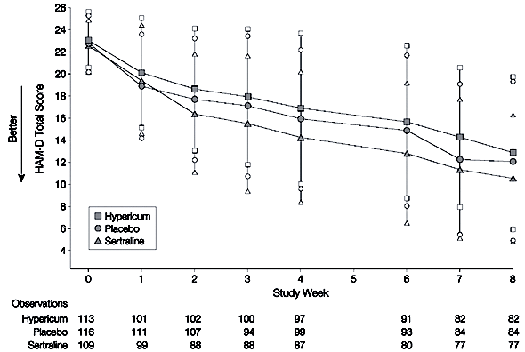
Graphed values are means with vertical bars extending to one
SD.
The authors report that the linear trends with time did not
differ significantly by treatment (St. John's vs. placebo p = .59, Zoloft
vs. placebo p = .18).
The results of the three treatments as related to clinical response
were:
| Response |
St. Johns wort (n = 113)
|
Placebo (n=116)
|
Zoloft (n=109)
|
| Any
response |
43.0 (38.1%)
|
50.0 (43.1%)
|
53.0 (48.6)%
|
| Full
response |
27.0 (23.9%)
|
37.0 (31.9%)
|
27.0 (24.8%)
|
| Partial
response |
16.0 (14.2%)
|
13.0 (11.2%)
|
26.0 (23.9%)
|
| No
response |
70.0 (61.9%)
|
66.0 (56.9%)
|
56.0 (51.4%)
|
While placebo had the highest full response, the authors report that there
were no significant differences in the full response between St. John's wort
and placebo (p= .21) or between Zoloft and placebo (p = .26).
Finally the authors give the estimated means for the improvements as measured
by the assessments scores. Recall that lower scores denote greater improvement
except for the GAF assessment.
|
Summary measure
|
St. John's wort
|
Placebo
|
Zoloft
|
St John's wort
Vs Placebo
p value
|
Zoloft
vs Placebo
p value
|
|
HAM-D total score
(week 8 - baseline)
|
-8.68
|
-9.20
|
-10.53
|
.59
|
.18
|
GAF score
(week 8 - baseline)
|
12.31
|
11.76
|
14.16
|
.75
|
.17
|
BDI total score
(week 8 - baseline)
|
-7.84
|
-6.83
|
-8.75
|
.43
|
.15
|
SDS total score
(acute exit - baseline) |
-3.34
|
-3.19
|
-4.01
|
.88
|
.39
|
CGI-S total score
(week 8 - baseline)
|
-1.07
|
-1.19
|
-1.47
|
.48
|
.11
|
|
CGI-I score
(week 8)
|
2.50
|
2.45
|
2.04
|
.75
|
.02
|
On all but one of the measures neither St. John's wort or Zoloft performed
significantly better than placebo. The exception was that Zoloft performed significantly
better than placebo on the CGI-I score.
The authors state their conclusion from this study as:
Conclusion. This study fails to support the efficacy of
St John's wort in moderately severe depression. The result may be due to low
assay sensitivity of the trial, but the complete absence of trends suggestive
of efficacy for St John's wort is notewworthy.
This conclusion and the headline of the NIH news release - Study shows St.
John's wort ineffective for major depresson of moderate severity - led to
similar headlines in the newspaper accounts of this study.
It seems to us that one could just as well replace St. John's wort by
Zoloft in both the authors' conclusion and the NIH headline.
Since studies have shown that Zoloft is more effective than placebo(1) and
the same is true for St. John's wort (2), the authors' suggestion that the trial
may not have had enough power to detect differences is probably correct.
The way this study was reported makes one worry about the role of subjectivity
in presenting the results of studies like this that involve controvertial methods
of treatment. The close connections researchers have these days with the subject
of their research suggests that this would be hard to avoid. One need only read
the following financial disclosure for the primary investigator Johathon R.T.
Davidson.
Financial Disclosure: Dr Davidson holds stock in Pfizer,
American Home Products, GlaxoSmithKline, Procter and Gamble, and Triangle Pharmaceuticals;
has received speaker fees from Solvay, Pfizer, GlaxoSmithKline, Wyeth-Ayerst,
Lichtwer, and the American Psychiatric Association; has been a scientific advisor
to Allergan, Solvay, Pfizer, GlaxoSmithKline, Forest Pharmaceuticals Inc, Eli
Lilly, Ancile, Roche, Novartis, and Organon; has received research support from
the National Institute of Mental Health (NIMH), Pfizer, Solvay, Eli Lilly, GlaxoSmithKline,
Wyeth-Ayerst, Organon, Forest Pharmaceuticals Inc, PureWorld, Allergan, and
Nutrition 21; has received drugs for studies from Eli Lilly, Schwabe, Nutrition
21, PureWorld Botanicals, and Pfizer; and has received royalties from MultiHealth
Systems Inc, Guilford Publications, and the American Psychiatric Association.
The financial disclosures of the other researchers are similar to this one.
DISCUSSION QUESTIONS:
(1) The authors say:
Sample-size calculations were based on detecting a difference
in full-response rates at 8 weeks, assuming full-response rates of 55% for hypericum
and 35% for placebo. Accordingly, a sample size of 336 patients (112 per group)
was specified to ensure 85% power with a type I error rate of 5% (2-sided).
Does this suggest that the study should have had sufficient power to detect
significant differences between the performance of St. John's wort and placebo
and Zoloft and placebo?
(2) Since the authors introduced Zoloft only to evaluate the study's sensitivity,
they did not include a comparison of the performance St. John's wort and Zoloft.
If they had, what do you think the result would have been?
(3) The design of the study in Biological Psychiatry (1) is quite similar
to the present study and yet it did show a significant difference between Zoloft
and placebo. Look at the two studies and see if you can explain how the difference
might have resulted.
REFERENCES:
(1) Setraline safety and efficacy in major depression," Fabre LF et al,
Biological Psychiatry. 38(9):592-602, 1995 Nov 1.
(2) St. John's wort for depression-an overview and meta-analysis of randomized
clinical trials, Linde K et al, British
Medical Journal 1996;313:253-258),
Height and earnings: Walk tall.
The Economist, 27 April 2002, 80
Al Gore was taller than George W. Bush, but in 10 of the last 13 presidential
elections the taller candidate has won. The article features a picture of Abe
Lincoln, our tallest president, along with a series plot comparing the heights
of US presidents with the average heights of white males at the corresponding
points in history. It does appear that presidents tend to be taller than average.
In the past, research has indicated that height is also an advantage in the
workplace. Three University of Pennsylvania economists recently investigated
this phenomenon using two large datasets, Britain's National Child Development
Study and America's National Longitudinal Study for Youth. You can download
the full 38 page pdf version of their
research report. As expected, height and earnings were positively associated.
Overall, for white British males, an additional inch of height was associated
with a 1.7% increase in wages; the corresponding advantage for white American
males was 1.8%. In both countries, the shortest quarter of workers averaged
10% lower earnings than the tallest quarter.
The intriguing twist in the new study is suggested by the article's subtitle:
"Why it pays to be a lanky teenager?" The researchers discovered that
most of the earnings advantage can be attributed to height at age 16. Differences
in height later in life or in childhood do not add much additional explanatory
power. The researchers proposed social adjustment as a possible explanation.
Taller teens may have an easier time participating in athletics and other activities,
where they develop positive self-esteem and social skills that contribute to
later success.
You can also listen to an interview
from ABC Perth (Australia), with Andrew Postlewaite, one of the study's three
authors. Postlewaite explains that the study focused on white males to prevent
confounding with gender and race effects. He reports that a height effect was
also found for women, but that the teenage height differences do not completely
explain adult earnings differences. For black males, the height effect was also
observed, but the sample was not large enough to give statistical significance.
DISCUSSION QUESTIONS:
(1) The article concludes with the following observation: "The differences
in schools and family backgrounds of tall and short youths are tiny compared
with those of white and black youngsters. If a teenage sense of social exclusion
influences future earnings, it may have great implications for youngsters from
minority groups." What implications do you see for minority groups?
(2) (Inspired by Rick Cleary) If the taller candidate has won ten of the last
thirteen elections, what do you suspect might be true of the last fourteen?
What are the implications for assessing whether there really is a height effect?
David Moore posted a to this article on the Isolated Statisticians
e-mail list.
Of canvases and coefficients:
New book uses statistical methods to analyze avant-garde art.
Chronicle of Higher Education, 19 April 2002, A20
Scott McLemee
What happens when statistics meets art history? University of Chicago economist
David Galenson found out that a quantitative perspective isn't always appreciated.
His new book Painting Outside the Lines: Patterns of Creativity in Modern
Art (Harvard University Press) is a statistical analysis of creativity in
avant-garde painting. He tried to publish his research in art journals, but
he reports that editors rejected his papers without even sending them out for
review.
Using regression analysis, Galenson identified two distinct forms of innovation:
"experimental" and "conceptual". The innovations of experimentalists,
such as Paul Cezanne, evolve gradually over time, as new techniques are developed
and refined. By contrast, artists like Pablo Picasso seem to innovate in quantum
leaps. Using the language of market economics, Galenson views artistic creativity
and skill as goods, for which artists are compensated with recognition in their
community. Many years later, such recognition translates into value placed on
the paintings (the artists themselves presumably may never see this). Galenson
found that the highest valuations for experimentalist paintings tended to be
for work produced towards the end of the artist's career, whereas conceptualists
tended to produce highly valued work earlier.
Predicting that critically acclaimed works will eventually command higher
prices may not sound controversial. The real shock comes from Galenson's claim
that by looking at price data he is able to use his model to "predict what
the artist said about his work and how he made preparatory drawings." This
may be too radical a conceptual shift for the art community. University of Kentucky
art historian Robert Jensen explains that scholars in his field see their work
as "the study of incommensurable art objects, these unique things in space and
time... . We've lost the capacity to generalize about the whole history
of art."
DISCUSSION QUESTION:
People want to be viewed as individuals, not as "statistics", which
can lead them to resist findings from epidemiological research. How does this
compare with the reaction that art historians are having to Galenson's work?
Do fingerprints lie?
The New Yorker, May 27, 2002, page 96
Michael Specter
According to the New Yorker article, "until this year, fingerprint evidence
had never successfully been challenged in any American courtroom." Then,
in January U.S. District Court Judge Louis H. Pollak issued a ruling that limited
the use of fingerprint evidence in a trial (U.S. v. Byron C. Mitchell) on the
grounds that fingerprint matching does not meet what are called "Daubert"
standards of scientific rigor. "Daubert" refers to a case-Daubert
vs. Merrill Dow Pharmaceutical-that the U. S. Supreme Court decided in 1993
in which the Daubert family sued Dow, alleging that a drug Dow manufactured
had caused birth defects. Expert scientific testimony had been presented by
the defense, but lower courts ruled such testimony did not meet "generally
accepted" standards. The U.S. Supreme Court was asked to clarify the requirements
for presenting scientific evidence in a trial, and in their ruling they identified
five conditions that must be met
- The theory or technique has been or can be tested.
- The theory or technique has been subjected to peer review or publication.
- Standards controlling use of the technique must exist and be maintained.
- The technique must have general acceptance in the scientific community.
- There must be a known potential rate of error.
As a result of this ruling, lawyers may request a "Daubert Hearing"
if they believe that the above standards should apply in a given case, but one
or more of the criteria have not been met. This is precisely what Mitchell's
defense lawyers did, arguing that fingerprint matching did not meet the standards--particularly
number 5. Although Pollak initially sided with Mitchell, on appeal he reversed
his decision. Nevertheless, the reliability of fingerprint evidence has never
received such public scrutiny and criticism. To this day there is no accepted
estimate for the probability that a portion of one person's fingerprint matches
a portion of another person's print, nor is there a known error rate in the
ability of finger print experts to identify a match.
Perhaps the most influential figure in the history of fingerprints is Sir Francis
Galton (1822-1911). To this day, the portions of a fingerprint deemed the most
important for identification purposes are called "Galton characteristics"
or "Galton minutiae". There are three main ridge pattern types that
appear on fingers: loops (~65%), whorls (~30%), and arches (~5%), and these
are further divided into subcategories. Roughly speaking, the minutiae are features
at the borders of the above types and subtypes, and are formed when ridges are
added or lost. For example, a ridge line may end abruptly, fork into two or
more lines, or join another line via a bridge. The presence (or absence, for
that matter) of Galton characteristics has been at the heart of virtually all
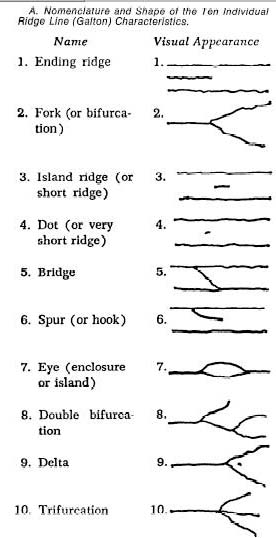
fingerprint identification methods. The article by Osterburg et al (1) provides
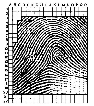
the following pictures of ridges in a fingerprint and the Galton characteristics.
 |
 |
Galton was also the first to quantify the uniqueness of fingerprints. In an
attempt to determine the chance that two fingers exhibit the same overall pattern,
he proceeded as follows. Using enlargements of fingerprint photographs, he let
square pieces of paper of various sizes fall at random onto the photographs.
Galton then attempted to fill in the squares, using only the ridge patterns
that he could see at the edges. His goal was to determine the size of a square
so that he could correctly infer the ridge pattern inside with probability .5.
Through repeated experiments he determined that the appropriate size was five
ridges on a side. There were 24 such regions per enlargement, so assuming independence
of the square regions, he calculated that the chance of obtaining a specific
print configuration, given the surrounding ridges, was
P(C/R) = (1/2)^24 = 5.96 x 10^(-8).
Galton next somewhat arbitrarily determined that P(R) = the chance that the
surrounding ridge pattern would occur = (1/16)(1/256); the first factor estimates
general fingerprint pattern type, and the second estimates the chance that the
appropriate number of ridges enter and exit the 24 regions. Using Galton's model
it follows that the probability of finding any given fingerprint is
P(FP) = P(C/R) P(R) = ((1/2)^24)(1/16)(1/256) = 1.45 * 10^(-11).
In Galton's day the world population was approximately 1.6 billion, yielding
16 billion fingers. Using the above figure he concluded that given a particular
finger, the chance of finding another finger with the same ridge pattern was
1/4.
A more recent approach by Osterburg et al (1) uses a similar overall method:
a fingerprint is overlaid with a grid of one millimeter squares as shown in
the figure above and each cell is either empty or contains one or more minutiae
(13 possibilities in all.) The difference here is that probabilities for each
of the 13 possible "states" for the cells are carefully estimated
through examination of actual prints. For example, an empty cell is by far the
most likely (76.6%), while a fork has observed frequency 3.82%. Again assuming
independence (this assumption is discussed later in the New Yorker article),
the probability of a particular configuration may be found by multiplying the
appropriate probability estimates.
Apparently most of the more recent studies have been ignored by the criminal
justice community.
Stone and Thornton (2) give an excellent discussion of the models proposed
by the time the article was written. You can read their critique of Galton's
method here. Galton's
method is in the spirit of today's "activities" and if it were used
as an activity it would be interesting to see if your class could decide whether
it should work nor not. We have not been able to decide this and would be interested
in hearing from any of our readers who might have opinions on whether Galton's
method should or should not work.
DISCUSSION QUESTIONS:
(1) Galton's model has been criticized by several authors. See a discussion
of Galtons model in (2)
here. Most find fault with Galton's assignment of a 1/2 probability of a
particular ridge configuration given a surrounding, five-ridge pattern. What
do you think? What happens if the region is shrunk to, say, one ridge square?
(2) Do you think Galton accepted the 1/4 figure? Do you?
(3) The Mitchell case raised questions concerning the abilities of fingerprint
"experts". (In fact in some studies a 22% false positive rate has
been observed.) How would you devise a test to determine a person's ability
to match whole or partial fingerprints?
(4) Do you think fingerprint evidence should be admissible in court? Why or
why not?
REFERENCES:
(1) Development of a Mathematical Formula for the Calculation of Fingerprint
Probabilities Based on Individual Characteristics, James W. Osterburg, T. Parthasarathy,
T. E. S. Raghavan, Stanley L. Sclove Journal of the American Statistical
Association, Vol. 72, No. 360. (Dec., 1977), pp. 772-778.
(2) A Critical Analysis of Quantitative Fingerprint Individuality Models, David
A. Stone and John I. Thornton Journal of Forensic Sciences, Vol. 31,
No. 4, Oct. 1986, pp. 1187-1219.
Are you suffering from security obsession syndrome?
Times (London), 5 May 2002
Peta Bee
Although violent crime has remained relatively rare in society, investments
in home alarm systems and self-defense training are on the rise. Spectacular
media coverage of crime may be partly to blame for fueling people's perception
that they are ever more at risk. According to the article, one in seven people
fear they will be mugged, while the British Crime Survey shows that only one
in 200 will actually become a victim.
Psychologists have coined the term "Security Obsession Syndrome"
(SOS) for the new preoccupation with safety. People are literally worrying themselves
sick. Health officials report that the stress associated with being constantly
on guard ultimately leads to physical symptoms, such high blood pressure and
cholesterol, backache, insomnia, and skin problems.
The article concludes with a number of recommendations to help people keep
a healthy perspective on crime. One victims' support group urges people to be
aware of their body language, because "We know from anecdotal evidence
that people who look vulnerable are more likely to attract attention and become
victims of crime."
DISCUSSION QUESTIONS:
(1) Over what time period do you think the one in 200 risk of being mugged
applies? Why does it matter?
(2) Do we ever "know" anything from anecdotal evidence? Can you
suggest any way to get a more scientific perspective on the last point?
The violence connection.
Washington Post, 26 May 2002, B5
Richard Morin
Children's groups have long warned of links between watching violent television
programs and violent behavior in real life. Research by L. Rowell Huesmann,
a social psychologist at the University of Michigan, confirms that these concerns
are well-founded. Moreover, Huesmann found that the adverse effects now apply
to girls as well as boys.
Huesmann's study began in 1977 with a group of 329 boys and girls, who were
then in elementary school. The investigators interviewed the children and developed
a measurement scale for television viewing that combined both time spent watching
and level of violence. Children in the top 20% were designated "heavy watchers."
In 1992, the investigators followed up with new interviews of the subjects,
who were now in their twenties. They also searched to find if any of the subjects
had criminal records.
After controlling for such variables as socioeconomic status and intelligence,
the investigators found that the "heavy watchers" had tended to become more
aggressive adults. As described in the article, women who had been heavy watchers
as children were twice as likely as the other women in the group to have hit
or choked another adult in the last year. Men who had been heavy watchers were
three times as likely to have been convicted of a crime. Among the women who
had married, the heavy watchers were twice as likely to have thrown an object
at their spouse in the last year. Among the men who had married, heavy watchers
were almost twice as likely to have grabbed or pushed their spouse in the last
year.
In 1999, Huesmann presented his case before a US Senate Committee on Commerce,
Science and Transportation. You can download a pdf
transcript of his testimony, "Violent video games: Why do they cause
violence and why do they sell?" There he draws parallels between violent
TV programming and tobacco. For example, he notes that both are widely distributed
and attractive to children; both have been linked to undesirable effects in
numerous longitudinal studies; and for both a dose-response relationship has
been observed. Nevertheless, in both cases our inability to conduct a controlled
experiment has allowed industry advocates to perpetuate doubts about any causal
link.
Data revised on soot in air and deaths.
New York Times, 5 June, 2002, A23
Andrew C. Revkin
Software glitch threw off mortality estimates.
Science, 14 June 2002, Vol. 296 No. 5575 p. 1945
Jocelyn Kaiser
The Health Effects Institute (HEI)
was established in 1980 as an unbiased research group to look into the health
effects of moter vehicle emissions. Their funding is typically one half from
the Environmental Protection Agency (EPA)
and one half from the automobile companies. Their research has concentrated
on determining the effect on health of small particles called particulated matter
(PM) in the air that we breath. These particles come primarily from industrial
plants such as steel mills and power plants, automobiles and trucks, and coal
and wood burners. Under the Clear Air Act established by Congress in 1970, the
EPA has developed regulations limiting the amount of partculated matter in the
air. The size of the particles involved is measured in microns (a micron is
a millionth of a meter). The regulations involve particulate matter up to 10
microns (PM10) called "coarse particles" and up to 2.5 microns (PM2.5)
called "fine particles". 10 microns is about 1/7 the diameter of a
human hair, and 2.5 microns is about 1/30 the diameter of human hair. Both coarse
and fine particles have been shown to cause health problems, but the fine particles
are particularly dangerous because they can so easily enter the lungs. More
information about particulate matter and the EPA regulations can be found here.
The studies that led up to the 1997 EPA regulations were typically time-series
studies on specific cities which identified an association between daily changes
in concentration of particulate matter and the daily number of deaths (mortality).
These studies also showed increased hospitalization (a measure of morbidity)
among the elderly for specific causes associated with particulate matter. However,
they did not demonstrate causality, and the limitation to specific cities left
questions about generalization to the general public. To help answer these questions
the HEI carried out a large study involving the 90 largest cities. They included
data on the amounts of other pollutants and the weather to determine if the
health effects could have other explanations. The results of their study were
reported in articles in the Royal Statistical Society, Series A, American Journal
of Epidemiology, New England Journal of Medicine and JASA. Detailed s
can be found here.
They concluded:
- There is strong evidence of an association between acute exposure to particulate
air pollution (PM10) and daily mortality, one day later.
- This association is strongest for respiratory and cardiovascular causes
of death.
- This association cannot be attributed to other pollutants including NO2,
CO, SO2 or O3 nor to weather.
- The average particulate pollution effect across the 90 largest U.S. cities
was a 0.41% increase in daily mortality per 10 microns per cubic meter of
PM10.
Recently, while looking again at their data, Scott Zeger found that when he
looked at data where he expected the SAS program to give different results it
did not. Here is an explanation of what was wrong as reported in Science.
They were using a model, the Generalized Additive Model (GAM), which is a multivariate
regression model particularly well suited to their problem of disentangling
the role of the particles from other confounding factors. The software carried
out an iterative process and was supposed to stop when the results did not differ
by epsilon. The default value for epsilon was 1/1000. However, the researchers
were dealing with tiny changes in daily rates and so should have used a smaller
value of epsilon. When they changed epsilon to a much smaller number they found
that they got slightly different results. Thus they had to redo all their calculations.
When they did this they found that the .41% increase in finding 4 became a 0.27%.
Thus they had a 34% decrease in their estimate of the overall increase in daily
mortality per 10 microns per cubic meter of PM10. The authors report that the
results related to mortality reported in items 1, 2, and 3 above remain valid.
The HEI has sent out a letter
acknowledging this error. You can see the results of this re-analysis here.
You will find here the following graphic for U.S. cities.
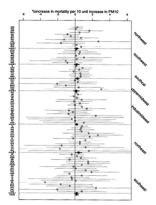
Maximum likelihood estimates and 95% confidence
intervals of the log-relative rates of mortality per 10 microns per cubic meter
increase in MP10 for each location. The solid squares with the bold segments
denote the posterior means and 95% posterior intervals of the pooled regional
effects. At the bottom, marked with a triangle is the overall effect for PM10
for 88 U.S. cities (Honolulu and Anchorage are excluded).
If you want to see if your city is here, you can obtain a pdf version of this
picture here which
can be enlarged to read the cities. However, you will still have to guess your
city's abbreviation.
Note that the overall effect, indictated by the line with a triangle at the
bottom of the graph, is just barely significant. The authors also present the
following more convincing graphic illustrating the results of a Bayesian analysis.
Marginal posterior distributions
for the re-analyzed pooled effects of PM10 at lag 1 for total mortality, cardiovascular-respiratory
mortality and other causes mortality, for the 90 U.S. cities. The box at the
top right provides the posterior probability that the overall effects are greater
than 0.
The Science article comments that this error gives new ammunition to industry
groups that have criticized the science behind the present federal air pollution
rules. It also serves as a warning to researchers that they need to completely
understand how a statistical package carries out its calculations. Obviously,
this experience of the Johns Hopkins researchers will lead other researchers
to take a second look at their results if they used the SAS GAM program.
DISCUSSION QUESTIONS:
(1) Will this discovery give support to those who claim that caution should
be used in Excel because of known errors in Excel calculations?
(2) The New York Times article states:
In the original analysis, the rise was .4 percent above the typical
mortality rate for each jump of 10 micrograms of soot per cubit meter of air.
In the new analysis, the increase is half that.
What would you like to know to get a better idea about the risk to you of particulate
particles? (See the next item).
Calculated Risks: How To Know When Numbers Deceive You.
Gerd Gigerenzer
Simon&Schuster, June 2002
Hardcover 288 pages, $17.50 at Amazon
There are two popular ideas on why the lay person has trouble understanding
probability and statistics reported by the media. One is that people who employ
statistics often have clever ways to lie with statistics. Another is that statistical
concepts are just too difficult for the general public to understand. The first
has led to a number of books that tell you how people lie with statistics (though
none quite as good as Huff's classic book How to Lie with Statistics).
The second has led to a number of books that try to teach the lay person standard
probability and statistical concepts using as few formulas and equations as
possible.
This book takes a different approach. The author suggests that the real problem
is that those who try to explain probability and statistics do not do so in
the way easiest for the public to understand. We found a striking example of
this while researching our previous article. We went to the researchers' web
site where we found an FAQ
page related to the error in determining the risk of small particles. Recall
that the researchers had reported a relative risk of 0.41% for mortality which
became 0.27% when the error was corrected. In the FAQ we read:
Question: But doesn’t the decrease from 0.41% to 0.27% represent
a 35% decrease in your assessment of the effect of PM10 on mortality?
Answer: Yes, this is one way to look at our result. However,
the implications may be less than is implied by a 35% reduction in the relative
rate. Although we use relative changes to measure the association of air pollution
with mortality for, public health purposes, it is the change in absolute risk
associated with pollution that is more important. In our case, the change in
risks due to implementing the full algorithm is 0.41-0.27=0.14% per 10 micrograms
per m3 of PM10.
To understand these changes, consider the city of Baltimore where
there are roughly 20 deaths per day or 7,300 deaths per year. If we could reduce
PM10 in Baltimore from the current average value of 35 down to 25 micrograms
per m^3, our prior estimate of 0.41% corresponds to saving 30 lives per year
from the acute effects alone. Our updated estimate would correspond to 20 deaths,
a change of 10 deaths per year.
The author of this book would ask: why not use the more informative method
for public health purposes?
A key theme of this book is that absolute risks are often more informative
than relative risk. Gigerenzer reports that women in Britain have gone through
several "Pill scares." For example, an official statement said that
"combined oral contraceptives containing desogestrel and gestoden are associated
with around a two-fold increase in the risk of thromboembolism (blockage of
a blood vessel by a clot). In terms of absolute risk the chance of thromboembolism
would be reported to increase from 1 to 2 in 14,000 women.
Note that the Johns Hopkins researchers also realize that results are better
understood when given in terms of frequency rather than probabilities, another
important theme of this book. Here is an example that is included in the book
based on an experiment carried out by Gigerenzer and Hoffrage (1). The authors
of this study asked 48 doctors to answer four different classical false positive
questions that would arise naturally in their work. One of these related to
screening for breast cancer. Here is how this example went. They were all told:
To facilitate early detection of breast cancer, women are encouraged
from a particular age on to participate at regular intervals in routine screening,
even if they have no obvious symptoms. Imagine you conduct in a certain region
such a breast cancer screening using mammography. For symptom-free women aged
40 to 50 who participate in screening using mammography, the following information
is available for this region.
The doctors were divided into two equal groups and assigned basically the same
question in two different forms. Half were given it in the "probability
format" and the other half in the "frequency format":
(probability format)
The probability that one of these women has breast cancer is
1%. If a woman has breast cancer, the probability is 80% that she will have
a positive mammography test. If a woman does not have breast cancer, the probability
is 10% that she will still have a positive mammography test. Imagine a woman
(aged 40 to 50, no symptoms) who has a positive mammography test in your breast
cancer screening. What is the probability that she actually has breast cancer?________%
(frequency format)
Ten out of every 1,000 women have breast cancer. Of these 10
women with breast cancer, 8 will have a positive mammography test. Of the remaining
990 women without breast cancer, 99 will still have a positive mammography test.
Imagine a sample of women (aged 40 to 50, no symptoms) who have positive mammography
tests in your breast cancer screening. How many of these women do actually have
breast cancer?_____out of______
Only 8% of those given the probability format got it right while 46% of those
given the frequency format got it right. The frequency format was the clear
winner in the other questions also. In discussing this experiment in another
article (2) Gegernzer included the following amusing cartoon of the two methods
for solving the problem:
Another theme of the book is the illusion of certainty. This occurs, for example,
in the courts with the claim that matches of ordinary fingerprinting and dna
fingerprinting demonstrate with certainty that the accused was at the scene
of the crime, in medicine with doctor's diagnosis of an ailment, and in almost
every presidential news conference. It is interesting to note that it also occurs
in the Gigerenzer-Hoffrage study (1) when they write "Ten out of every
1,000 women have breast cancer. Of these 10 women with breast cancer, 8 will
have a positive mammography test".
Another major theme in this book is risk and making decisions in the face of
uncertainty. The author illustrates the many issues here by a case study of
screening for breast cancer. The author has clearly done his homework presenting
very up-to-date information of the many studies that have been carried out related
to screening for breast cancer. We can think of no better example to show the
difficulties in making decisions in the face of uncertainty. Here a false positive
can lead to serious depression, further invasive testing, and unnecessary medical
treatments. This example provides a wonderful laboratory for all the author's
ideas on how best to communicate to doctors and patients what studies have and
have not shown about breast cancer screening. See the next item for an elegant
application of the methods discussed in this book applied to presenting cancer
risks.
If this book is widely read it will make a significant contribution to statistical
literacy. The author has made a strong case that probability and statistical
information is not presented to the lay person in the right way and has made
recommendations on how this can be improved. The book is completely accessible
to the lay person and will give him or her a new appreciation of the role of
probability and statistics in making decisions under uncertainty in daily life.
Reading this book will also help researchers, doctors, and news writers transmit
information in a way that will be most helpful to the general public. Finally,
it will give teachers a new perspective on teaching probability and statistics
in a way that will stay with their students when it is their turn to face decisions
under uncertainty.
Of course, no single book can be expected to solve this problem. However, it
is surprising how little has been done to improve statistical literacy in the
general public and "Calculated Risk: How to Know When Numbers Deceive You"
should make a significant contribution toward such improvement.
DISCUSSION QUESTIONS:
(1) Some say that stating a problem using the frequency format is, to some
extent, giving away the answer. What do you think about this claim?
(2) Would you be concerned that given results of experiments using the frequency
format would give the public a false sense of variations in statistics? If so,
how could we guard against this and still use the frequency format?
(3) Why do you think researchers and news writers tend to prefer relative risk
to absolute risk?
REFERENCES:
(1) Hoffrage, U., and G. Gigerenzer. 1998. Using natural frequencies to improve
diagnostic inferences. Academic Medicine 73(May):538.
(2) The psychology of good-judgment, Gerd Gigerenzser, Medical Decision
Making, 1996;3;273-280.
The H.G. Wells Quote on statistics: a question of accuracy.
Historia Mathematica 6 (1979), 30-33
James W. Tankard
Gerd Gegerenzer starts and ends his book "Calculated Risks" with
two famous quotations:"...in this world there is nothing certain but death
and taxes", attributed to Benjamin Franklin, and "Statistical thinking
will one day be as necessary for efficient citizenship as the ability to read
and write", attributed to H. G. Wells.
Gigerenzer calls the first quote "Franklin's law". About the second
quotation, he writes in his notes:
This statement is quoted from How Lie with Statistics
(Huff, 1954/1993), where it serves as an epigraph. No is given. I
have searched through scores of statistical textbooks in which it has since
been quoted and found none where a was given. I could not find this
statement in Wells' work either. Thus, the source of this statement remains
uncertain, another example of Franklin's law.
We could not resist the challenge to find the origin of this famous quotation.
Its origin is described by in this article by Tankard. It turns out to be another
example of statistics stealing from mathematics. Tankard states that the earliest
occurrence of the quotation in writings about statistics is as an epigraph at
the beginning of Helen M Walker's Studies in the History of Statistical Method
(1929),
The time may not be very remote when it will be understood that
for complete initiation as an efficient citizen of one of the new great complex
world-wide States that are now developing, it is as necessary to be able to
compute, to think in averages and maxima and minima, as it is now to be able
to read and write.
and attributed it to H.G. Wells book Mankind in the Making. Tankard
states that this is part of a longer sentence in this book:
The great body of physical science, a great deal of the essential
fact of financial science, and endless social and political problems are only
accessible and only thinkable to those who have had a sound training in mathematical
analysis, and the time may not be very remote when it will be understood that
for complete initiation as an efficient citizen of one of the new great complex
worldwide States that are now developing, it is as necessary to be able to compute,
to think in averages and maxima and minima, as it is now to be able to read
and write.
In other words, Walker left out the to a need for a sound training
in mathematical sciences. Apparently, "Statistical thinking" first
occurred in the quote from Sam Wilks' presidential address to the American Statistical
Society "The Teaching of Undergraduate Statistics" (1). Here we find
the statement:
Perhaps H. G. Wells was right when he said "Statistical
thinking will one day be as necessary for efficient citizenship as the ability
to read and write!"
Thus the takeover was completed! Tankard remarks that statistics does not occur
in the index in any of Wells' autobiographies and biographer Lovat Dickson told
him that he could not recall any place in Wells' writings where he dealt specifically
with statistics.
Incidentally, it is interesting to compare the discussion of undergraduate
statistics courses in Wilk's Presidential address with that in David Moore's
1998 Presidential address Statistics
among the Liberal Arts on a similar topic. For example, The word data
occurs once in Wilks' address and 53 times in Moore's.
REFERENCES
(1) S. S. Wilks, Undergraduate statistical education, JASA,Vol.
46, No. 253. (Mar., 1951), pp. 1-18.
Experts strive to put diseases in proper perspective.
New York Times, 2 July 2002, D5 (Science Times)
Gina Kolata
Risk
Charts: Putting cancer in context.
Journal of the National Cancer Institute, Commentary, Vol. 94, No. 11, June
5,2002
Steven Woloshin, Lisa M. Schwartz, H. Gilbert Welch
The New York Times article has a good discussion of the need for better ways
to present statistical information to the public. This includes issues like
relative risk vs absolute risk, how population risks should be interpreted by
individuals, probabilistic vs. frequency methods to give odds etc. The commentary
by Woloshin and his colleague uses the frequency approach to provide an impressive
chart to help people decide on risks of cancer. This is reproduced in the New
York Times article in the following elegant form:
Looking at the column for your age, you can find the number of people per 1000
who will be expected to die from a variety of causes depending on whether you
are a smoker or not. For each disease, the top row is for a non-smoker and the
bottom row for a current smoker. Looking at the age 80 Laurie finds that his
biggest worry is a heart attack. Charles, looking at age 50 has to begin worrying
about heart disease, and Bill looking at 45 and Jeanne at 40 really don't have
much to worry about as long as they don't take up smoking. So Laurie will quit
playing tennis in 90 degree weather, Charles will watch his colesterol, and
Bill and Jeanne will enjoy the good life while it lasts.
Gina Kolata (1) recently had a chance to apply the recommendations from her
previous article. She wrote about a recent article in JAMA (3). reporting a
major study on the benefits to women of replacement therapy that was haltled
because the risks appeared to be greater than the benefits.Kolata writes:
The data indicate that if 10,000 women take the drugs for a year,
8 more will develop invasive breast cancer, compared with 10,000 who were not
taking hormone replacement therapy. An additional 7 will have a heart attack,
8 will have a stroke, and 18 will have blood clots. But there will be 6 fewer
colorectal cancers and 5 fewer hip fractures.
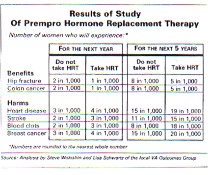
In an article in our local newspaper (2), Steve Woloshin and Lisa Scharwtz
presented the following more informative table based on data from the JAMA.
The average time of follow up in this study was 5.2 years.
DISCUSSION QUESTIONS:
(1) The Science Times article quotes Steven N. Goodman, an epidemiologist
at Johns Hopkins School of Medicine as saying:
One way to think about risk is that each of us has a little ticking
time bomb, a riskometer inside us. It says that everyone is at risk and that
eating and health habits can raise or lower risk.
The other way comes closer to the way many people experience
risk. It says that the risk is not to them but that each individual has a fate.
I'm either going to survive this cancer or not. Probabilities are uncertainties
that the doctor has about what is going to happen to us. And that is a profoundly
different way of thinking about risk.
The complication is that probability has both of these meanings
simultaneously.
Which way is closest to how you think about risk? How would you describe the
way you look at risk?
(2) The Science Times article reports that Dr. David McNamee, an editor
at the Lancet, sent an e-mail to Woloshin saying the charts work for him and
commenting:
Foolishly, I started smoking again last year after quitting for
about 20 years. I can see it is time to stop again (I am 50 in November), and
get back to the gym. I have put the charts on the office wall.
What would be your estimate for the number of people who would quit smoking
after looking at this chart in the Science Times article?
(3) What is the problem with the way Gina Kolata explained the risks of homone
replacements?
REFERENCES:
(1) Citing Risks, U.S. Will Halt Study of Drugs for Hormones, The New York
Times, 9 July 2002, A1, Gina Kolata.
(2) Hormone Study Starts Scramble, Valley News, 13 July, 2002, A1, Krinstina
Eddy
(3) Risk and Benefits of Estrogen plus Progestin in Healthy Postmenopausal
Women, Writing Group for the Women's Health Initiative Investigators, JAMA,
Vol. 288 No.3, July 17, 2002
We received the following letter from our colleague Larry
Polansky in the Dartmouth Music Department.
Dear Chance News
I'm a musician with a strong interest in mathematics, and I recently performed
a piece which involved probability as a kind of essential element to the work.
The piece raises a probability question (which I don't know the answer to) that
I thought would be fun to readers of this newsletter.
The piece was by Seattle composer David Mahler, and it was a trio for mandolin,
flute, and piano. It was called "Short of Success." It was part of
a larger work called "After Richard Hugo", for five musicians. The
trio was based on the idea that one should embrace lack of perfection as a necessary
component of poetry, but nonetheless strive for perfection.
Here's the way the piece worked. There were nine single pages of score, each
a single melody. Each page was a slightly different version of every other page.
Each of the three musicians had the same set of nine pages. Before the performance,
each of the three musicians "randomly" rearranged their pages, independently
of the other two musicians. We then played each page, in unison, until we heard
a "discrepancy." At that point, we stopped and moved on to the next
page. The instructions for the piece were that if we ever played the same page
(which would have resulted in a single unison melody), the person who started
that particular page (each new page is cued by one of the musicians) was supposed
to shrug their shoulders, and say, without enthusiasm: "success".
My question is: what are the odds of that actually occurring? Needless to say,
in four or five performances of the work, and in maybe 20-30 times rehearsing
it, it never occurred.
Larry Polansky
Music Dept.
Dartmouth College
Larry sent us the music, instructions for playing it, and a performance of
the piece at Dartmouth. To better understand the music and the problem we recommend
that you print the instructions and version 1 and then listen to the Dartmouth
performance of the composition. You can find these here
Dartmouth
performance, Instructions
for playing, version
1,version 2,version
3,version 4,version
5,version 6,version
7,version 8,version
9.
Of course if you happen to have three musicians handy it would be better yet
to make copies of all the versions and play the piece yourself.
Here is our solution to his problem.
We assume that the composer labels the 9 versions from 1 to 9. Each player recieves
a copy of these nine versions. They mix up their copies and play them in the
resulting order. The numbers on the music of a player in the order the versions
are played is a random permutation of the numbers from 1 to 9. If the resulting
three permuations have the same number in a particular position, we call this
a "fixed point" of the three permutations. The players will have success
if there is at least one fixed point in the three permutations. For example,
if the labels in the order they were played are
| piano |
2
|
4
|
6
|
5
|
9
|
3
|
7
|
1
|
8
|
| mandolin |
5
|
8
|
1
|
6
|
9
|
3
|
7
|
4
|
2
|
| flute |
1
|
6
|
8
|
3
|
2
|
9
|
7
|
4
|
5
|
then 7 is a fixed point and the trio would have success on the 7th run through
of the piece.
Thus Larry's question is: If we choose 3 random permutations of the numbers
from 1 to 9, what is the probability that there is at least one fixed point?
Since Larry also mentions a larger composition with 5 instruments we will generalize
the problem by assuming that there are m players and each player has n versions
of the composition. Then our problem is: If we choose m random permutations
of the numbers from 1 to n, what is the probability that there is at least one
fixed point?
The case of two players, m = 2, is equivalent to one of the oldest problems
in probability theory now called the "hat-check" problem. In this
version of the problem, n men check their hats in a restaurant and the hats
get all scrambled up before they are returned. What is the probability that
at least one man gets his own hat back? What is remarkable about this problem
is that the answer is essentially constant, 1 - 1/e = 0.632121... for any number
of men greater than 8.
The proof of this result can be found in almost any probability book, for example
on page 104 of the book "Introduction to Probability" by Grinstead
and Snell, available on the web here.
The proof uses the familiar inclusion-exclusion formula. The proof of our more
general case is similar and can be found here.
Here are the probabilities for success with 2 players, 3 players, and 5 players
when the number versions varies from 2 to 10.
|
no.of versions
|
2 players
|
3 players
|
5 players
|
|
2
|
.5
|
.25
|
.0625
|
|
3
|
.667
|
.278
|
.035
|
|
4
|
.625
|
.214
|
.015
|
|
5
|
.632
|
.178
|
.008
|
|
6
|
.633
|
.151
|
.005
|
|
7
|
.632
|
.132
|
.003
|
|
8
|
,632
|
.117
|
.002
|
|
9
|
.632
|
.104
|
.001
|
|
10
|
,632
|
.095
|
.001
|
Probability of success.
Note that when we have 5 players, the probability of success decreases rapidly.
The best probability of success in this case would be a 6 percent chance of
success when there are only 2 versions of the piece. There would be only a 1.5
percent chance of success with 4 versions and with 9 versions the players would
probability never have success. We see that for Larry's question (m = 3, n =
9) the answer is that the probability of success is .10445. Thus Larry's group
should expect to succeed about 1 in 10 times they rehearse or play "Short
of Success." Larry expressed surprise with this result writing:
Does that mean the probability of success (.104) is about 1 in
ten? that's
MUCH higher than I expected, and (not really evidence) much higher than our
actual experience (we performed the piece 5 times, rehearsed it maybe 15-20,
and
never had "success")
We suggested that the problem might be with false positive or false negative
results. A false positive result could occur, for example, if on a particular
run through two players have the same version, the third player has a version
which is very close to their version and the difference is simply not noticed.
A false negative would occur if on a particular run through they all have the
same version but a player hits a wrong note which is interpreted as a difference
in his version. The false-positive and false-negative rates could be estimated
if the players would keep a record of their permutations and what actually happened
when they played the piece. We asked Larry what he thought about this and he
replied:
Re: false positive and false negative. That, in fact, is integral,
I think, to the musical notion of the piece. It's fairly hard for three musicians
to always play perfectly in unison without making a mistake (it's a reasonably
difficult page of music), and we had LOTS of situations where we weren't sure
if it was "us" or the "system." That not only confirms what
you hypothesize (that we may have, in fact, "hit it" several times
without realizing it), but it is also very much, I think, part of the aesthetic
of the work, which investigates the notions of success, perfection, and failure
in wonderful ways.
Your formulation of the problem gives some nice added richness
(or perhaps I should say, resonance) to the piece itself which I'm sure David
is enjoying immensely. I would say (in our defense, since musicians never want
to admit to clams) that most of the time when that happened, and we were suspicious,
we asked each other "which number did you have up on the stand?" and
every single time (strangely), we had different ones. But I can't swear that
we ALWAYS confirmed it in this way.
Thanks again, the description is great, the answer fascinating,
and completely changes my perspective of a piece that I just performed a number
of times!
We received the following suggestion from Roger Johnson
at the South Dakota School of Mines & Technology for Chance News:
In Dean Koontz's novel From the Corner of His Eye Jacob shuffles four
decks of new cards. Maria then draws 12 cards - 8 aces followed by 4 jacks of
spades. What is the chance of this? Later, we find that Jacob is a "card
mechanic" and has deliberately shuffled the decks to produce the first
8 aces but not the 4 jacks of spades:
The odds against drawing a jack of spades four times in a row
out of four combined and randomly shuffled decks were forbidding. Jacob didn't
have the knowledge necessary to calculate those odds, but he knew they were
astronomical." [p. 234]
With the understanding that the aces were arranged to be drawn first but that,
beyond this, the cards were randomly arranged, what is the chance that the 4
jacks of spades are then drawn? In the novel, 2 cards are set aside between
drawings so that 22 cards have been drawn at the time the eighth ace is drawn
(and, so, 4*52 - 22 or 186 cards remain).
Regarding this strange draw of cards the author writes:
Not every coincidence, however, has meaning. Toss a quarter one
million times, roughly half a million heads will turn up, roughly the same number
of tails. In the process, there will be instances when heads turn up thirty,
forty, a hundred times in a row. This does not mean that destiny is at work
or that God - choosing to be not merely his usual mysterious self but utterly
inscrutable - is warning of Armageddon through the medium of the quarter; it
means the laws of probability hold true only in the long run, and that short-run
anomalies are meaningful solely to the gullible. [pp. 200-201]
Schilling's (1990) article "The longest run of heads" in the College
Mathematics Journal (vol. 21, pp. 196-207) gives the result that in n tosses
of a fair coin the expected longest run of heads is nearly ln n/ln 2 - 2/3 with
a standard deviation of nearly 1.873 (constant in n). Given this, what do you
think of the quote above from Koontz's novel about seeing heads "thirty,
forty, a hundred times in a row" in a million tosses? Would you say that
Koontz is correct "in spirit"? Why? (Read Schilling's article.
Bob Johnson at Monroe Community College sent us the following
note about the Beyond
the Formula Statistics Conference held every year at Monroe Community
College in Rochester New York. We note that this year's keynote speaker is Joan
Garfield a long time member of the "Chance team." Bob writes:
August 8 & 9, 2002. Save those dates!!
Plan to attend the 6th annual Beyond The Formula Statistics Conference,
“Constantly Improving Introductory Statistics: The Role of Assessment.”
As always the program features topics in the areas of curriculum, teaching techniques,
technology usage, and applications along with this year’s thread topic
Assessment.
Speakers include: Joan Garfield (Keynote), James Bohan, Beth
Chance, Mark Earley, Patricia Kuby, Allan Rossman, John Spurrier
For detailed Information, please visit our web
site.
Professor Edward Kaplan sent us a correction to our discussion
in Chance News 11.02 of the following article:
Hi -- by "chance" I came across your newsletter, which
just happened to mention my Op Ed on travel risks to Israel.
You have one of the numbers wrong -- as did the Jerusalem Post
-- the copyeditor changed some figures AFTER I had returned my last version.
They corrected it, so now some online versions of the J. Post have the right
numbers and some the wrong! However, the numbers in the OR/MS Today version
were correct.
I bet some of your readers saw the inconsistency -- 120 deaths
over 442 days in a population of 6.3 million does NOT work out to a death risk
of 19 per million (per year!). It works out to a risk of 120 * (365.25/442)
/ 6.3 = 16 per million per year.
At the time I wrote this, I believed I was being conservative
-- the 442 days I included were during a period of above-average terror attacks
(in both frequency and casualties). Sadly things have gotten worse -- but even
if you were to substitute more recent statistics, you would still find the death
risk from driving in the US to be just as scary. There is no question that people
overestimate the risk of being a terror victim -- just like people overestimate
the chance of winning the lottery. The nature of rare events is that, while
one can happen every day, the likelihood of one happening to YOU on a given
day is very, very small.
Edward H. Kaplan, Ph.D.
William N. and Marie A. Beach Professor of Management Sciences
Professor of Public Health
Yale School of Management
Professor Kaplan has also sent us two papers that we think Chance
readers and students would enjoy.
The first is a working paper entitled A New Approach to Estimating the Probability
of Winning the Presidency written with Arnold Barnett. Readers will
recall that Arnold Barnett gave one of our first and favorite Chance
Lectures.
Abstract:
As the 2000 election so vividly showed, it is Electoral College standings rather
than national popular votes that determine who becomes President. But current
pre-election polls focus almost exclusively on the popular vote. Here we present
a method by which pollsters can achieve both point estimates and margins of
error for a presidential candidate's electoral-vote total. We use data from
both the 2000 and 1988 elections to illustrate the approach. Moreover, we indicate
that the sample sizes needed for reliable inferences are similar to those now
used in popular-vote polling.
You can obtain the full text version of this paper here.
The second paper is March Madness and the Office Pool, co-authored with
Stanley J. Garstka, which appeared in Management Science Vol. 47, No. 2, March
2001, pp. 369-382.
Abstract
March brings March Madness, the annual conclusion to the US men's
college basketball season with two single elimination basketball tournaments
showcasing the best college teams in the country. Almost as mad is the plethora
of office pools across the country where the object is to pick a priori as many
game winners as possible in the tournament. More generally, the object in an
office pool is to maximize total pool points, where different points are awarded
for different correct winning predictions. We consider the structure of single
elimination tournaments, and show how to efficiently calculate the mean and
the variance of the number of correctly predicted wins (or more generally the
total points earned in an office pool) for a given slate of predicted winners.
We apply these results to both random and Markov tournaments. We then show how
to determine optimal office pool predictions that maximize the expected number
of points earned in the pool. Considering various Markov probability models
for predicting game winners based on regular season performance, professional
sports rankings, and Las Vegas betting odds, we compare our predictions with
what actually happened in past NCAA and NIT tournaments. These models perform
similarly, achieving overall prediction accuracy's of about 58%, but do not
surpass the simple strategy of picking the seeds when the goal is to pick as
many game winners as possible. For a more sophisticated point structure, however,
our models do outperform the strategy of picking the seeds.
You can obtain the full text of this paper here.
Don Poe at the American
University sent us the following note:
Laurie -
I love Chance News and often use it as the source of materials
for my statistics courses. I do, however, want to comment on an item in the
current edition (11.02).
Item #10 contains a brief comment by Marilyn vos Savant about
the fairness of deciding important sports outcomes by a coin toss. In an addendum
she says that such decisions could still be fair, "even if the coin were
two-headed or two-tailed, as long as the team that chooses has no information
about the coin." Loathe though I am to ever disagree with Marilyn (statisticians
who do usually end up with egg on their face), in this case I think I would
at least want to add a qualification to her answer. That is, this odd situation
would be fair if the team doing the choosing did so completely randomly. But
I personally doubt that this is true of human nature.
Imagine the following situation (it's more than a bit contrived,
but bear with me): Dartmouth and Princeton are playing football for the Ivy
League championship. The game is tied after regulation and the rules require
a sudden death playoff where the first team to score wins the game. The teams
are about to have a coin toss to see who gets the ball first, in this case obviously
a tremendous advantage. The unscrupulous referee secretly has a huge bet on
the game's outcome and will stand to win big if Dartmouth wins the game. In
his pocket he has 3 coins - a fair coin, a two-headed coin and a two-tailed
coin. When he is not refereeing Ivy League football games this man is a sports
psychologist who recently read an empirical article that shows that in coin
tosses, the team doing the choosing tends to pick heads significantly more often
than tails. If Dartmouth is calling the coin toss, he uses the two-headed coin
under the assumption that Dartmouth is at least slightly more likely to call
heads. If Princeton calls the toss, he uses the two-tailed coin for the same
reason. According to Marilyn, the referee's choice of the coin to toss could
not possibly have an impact on the outcome since the person calling the toss
has no information. If the empirical article is right (i.e., people do not call
coin tosses randomly), then she is wrong and the referee has changed the odds
in favor of Dartmouth.
This reminded us of the activity that our colleague Psychologist George Wolford
did in our Dartmouth Chance class. He said that he understood that the class
had tried ESP experiments and they seemed not to have extrasensory perception.
However, he would show them that they did. He put down five coins in a row and
wrote the sequence of heads and tails on a piece of paper that he put in a sealed
envelope. He then asked the students to think very hard and write down what
they thought his sequence was. Then he wrote each person's sequence on the board
and, lo and behold, the correct sequence was the most popular answer.
Copyright (c) 2001 Laurie
Snell
This work is freely redistributable
under the terms of the GNU
General Public License published
by the Free Software Foundation.
This work comes with ABSOLUTELY NO
WARRANTY.
CHANCE News 11.03
21 April 2002 to 13 July 2002