The current and previous issues of Chance News and other materials for teaching a Chance course are available from the Chance web site.
Chance News is distributed under the GNU General Public License (so-called
'copyleft'). See the end of the newsletter for details.
I would like to believe, that if someone studies these things a little more closely, then he will almost certainly come to the conclusion that it is not just a game which has been treated here, but that the principles and the foundations are laid of a very nice and very deep speculation.
Huygens referring to his treatise
"On Reasoning in Games of chance" 1757
Contents of Chance News 12.03
1.
Chance News contributes a Forsooth item.
2.
So much for not being statistically significant!
3. A new Chance News for news reports of medical studies.
4.
Random matrices and the Riemann Hypothesis are in the news.
5. Area-fault study estimates 62% chance of deadly 6.7 tremblor.
6.
The Bush doctrine: How many wars are in us?
7. Marilyn on the chance of being struck by lightning vs the
chance of winning the lottery.
8. Do companies named foo.com do better if they drop the .com?
9.
What some much-noted data really showed about vouchers.
10.
A mathematician crunches the Supreme Court's numbers.
11.
Brian Hayes answers a coincidence problem.
12. What does "chance" mean?
13. Maybe we should also ask what" probability"
means.
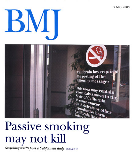
14. New study claims secondhand smoke is not a serious risk
factor for heart attacks.
15.
Why does Zipf's law play such an important role in languages?
Jerry Grossman sent us a Forsooth item that we created in our last Chance News (12.02).
We wrote:
Those who set odds for betting usually assume that the proportion of money bet on an outcome is a good estimate for the probability that the outcome will occur. Assuming this is the case, then the probabilities would add up to 1. If these probabilities were used to create the odds, then the expected profit would be $0. On the other hand, if we multiply the probabilities by 1.2, making their sum 1.2, and use these to determine the odds, the expected profit will be about 20% of the money bet which is about what bookies want.
Jerry wrote:
I don't think the bookie's profit is 20% of the money bet. Let's take a simpler example. There are three horses, each with 1/3 chance of winning. The odds are stated as even money for each horse. So the sum of the probabilities is 1.5. One person bets $1 on each horse, for a total of $3. The bookie keeps the $2 from the losers and returns the $1 bet plus $1 to the winner. So the bookie has made a profit of $1, which is 33% of the total amount bet, not 50%.
He is correct!
Judy Soukup sent us the following note:
In the Washington Post of May 27, 2003, titled "Miracle Cure? Fat Chance", there is a lovely, typical forsooth. The italics are mine:
Calories count. The Atkins philosophy is that total calories consumed don't matter, provided carbohydrates are severely restricted. But in one of the studies published last week, participants in the Atkins group ate fewer calories than those in the low-fat group, although the differences were not statistically significant. "The law of thermodynamics still holds here," says Frederick Samaha, chief of cardiology at the Philadelphia Veterans Administration Hospital and lead author of the study. "Weight loss is still entirely an effect of total calories in and total calories out."
So much for not being statistically significant!
The National electronic Library for Health Programme is working with the National Health Service libraries to develop a digital library for the NHS staff, patients and the public. This library can be found at the NeLH website. Of interest to us is a column called "Hitting the Headlines." Here the question "should we believe it?" is asked for a current medical issue in the news. Here is the current issue as this was written:
'Hand-held scanner could detect tumours'Two newspapers reported the development of a hand-held scanner that 'frisks' patients to detect cancer tumours. Promising results for prostate cancer were quoted. The research on which these claims were based had not been published and so it was not possible to comment on their accuracy.
This report has been prepared for the National electronic Library for Health by the NHS Centre for Reviews and Dissemination, based at the University of YorkReferences and resources1. The cancer 'frisker'. Daily Mail, 12 June 2003, p41. 2. Airport-style cancer scan. The Sun, 12 June 2003, p16. 3. Hand-held scanner could detect tumours. New Scientist, 14 June 2003, p15. |
Previous issues are archived here.
Brian Hayes writes a regular column "Computing Science" for the American Scientist. Readers of Chance News will recall his two fine articles, one on Louis Freye Richardson as the first weather forecaster and another on Richardson's attempt to use statistics to try to understand the causes of war (see Chance News 11.04) as well as Brian's article on randomness discussed in Chance News 9.04. In his current column, Brian writes about the connection of random matrices to the Riemann Hypothesis. This should not be a new subject to readers of our Chance in the Primes, but Brian is an excellent science writer and you are guaranteed to learn something new from his articles. This is a timely contribution for readers of the three popular books on the Riemann Hypothesis that have appeared recently.
In the same issue of the American Scientist, Enrico Bombieri reviews two of the new books on the Riemann Hypothesis: "Prime Obsession" by John Derbyshure and "The Riemann Hypothesis" by Karl Sabbagh. Bombieri is one of the leading number theorists who has himself worked on the Riemann Hypothesis. Bombieri wrote a nice account of the history of the Riemann Hypothesis for the Clay Mathematical Institute which is offering a million dollar prize to the person who solves this problem. Of course, Derbyshure and Sabbagh have to go easy on the math; so you might want to keep Bombieri's account by your side when you read one of these books, in case you want to know more precisely the mathematical background of the Remann Hypothesis.
In addition to alerting us to these articles, Brian sent us an account of his discussion with a friend who asked: what is the chance of that? In this case the "that" was: In the 2002 elections in Comal County Texas, the winners of three of 30 county wide races had exactly the same number of votes, namely 18181. You will find how Brian answered his friend later in this issue of Chance News. For his answer Brian needed to determine the probability of three or more people having the same birthday. This is not as easy as the classical problem of finding the probability that two or more people have the same birthday.
A group of more than one hundred earthquake experts from federal and state agencies, universities and earthquake engineering firms have collaborated to assess Northern California's earthquake risk. Their work combines the latest seismic data with state-of-the-art computer models to predict earthquake damage. The headline announces the main finding: there is a 62% probability of a magnitude 6.7 or greater quake striking the area within the next 30 years. The Chronicle quotes David P. Schwarz of the U.S. Geological Survey as saying:
Our new data now is much more sophisticated and much more robust, but our results must still reflect many uncertainties. So we have to accept a broad error range, which could be anywhere from 38 percent to 87 percent, considering many different earthquake theories -- which poses a big uncertainty. What we do know for sure, however, is that any big earthquake in the Bay Area will produce damaging ground motions over broad areas, and at substantial distances from the source of the quake.
The U.S. Geological Survey maintains a Earthquake Hazards Website, where you can find technical summaries, news releases, and data graphics from the probability study. There is also a link to a webcast of a 70-minute lecture entitled "Bay Area Earthquake Probabilities", which was sponsored by the University of California at Berkeley's Seismological Lab.
DISCUSSION QUESTIONS:
(1) The article states "there is a 62 percent probability of a
major quake with a magnitude greater than 6.7 striking the region before
the year 2032. There is a more than 80 percent likelihood that a smaller
but still very damaging temblor of magnitude 6 to 6.6 will strike here
during that time period, the scientists agreed." But do you agree?
Is it clear how to straighten this out?
(2) The Los Angeles Times (Scientists lower estimated chance of major Bay Area quake. 23 April 2003, Part 2, p. 6) described the findings this way: Scientists said that while using the 62% overall figure, they can be 95% sure that the probability of a 6.7 quake or larger in the next 30 years ranges between 37% and 87%. But two paragraphs later we read: The 37% to 87% span of probabilities reflected differences between four separate seismic models used, with the lowest close to 37% and the highest close to 87%. Can these both be correct?
Vasquez is the author of The War Puzzle (Cambridge University Press, 1993), in which he proposes to investigate scientifically the causes and results of war. In the present article, he summarizes some of his arguments as they apply to the Bush Administration's approach to confronting terrorism.
Vasquez emphasizes the distinction between "preemptive" and "preventive" wars. The former are intended to undermine an imminent attack by striking first. The latter are undertaken to prevent a hostile regime from even developing the capability to mount an attack. The current US approach to terrorism seems to require a series of preventative strikes. Having just succeeded in Iraq, we have recently issued warnings to both Syria and Iran. Vasquez warns that we cannot count on victory in every such engagement. He cites one statistical study of wars fought from 1816 to 1945, which found that the state that was wealthier and lost a smaller percentage of its population prevailed 84% of the time. While the US seems to enjoy these advantages, Vasquez wonders if anyone is paying attention to the 16% downside.
Furthermore, we cannot count on every conflict being decided quickly. Vasquez cites studies of Korean and Vietnam wars to show that at each point where US casualties increased by factors of 10 (from tens to hundreds to thousands), public support dropped significantly. Falling below a 50% approval rating has obvious political ramifications. Vasquez notes that the time it takes to reach this point depends on the level of public support at the start of the operation. He predicts that a prolonged series of wars will steadily diminish the public's will to fight.
DISCUSSION QUESTION:
Describing the hazards in a series of operations, Vasquez writes: But what works
once, twice or even three times might not continue to work... . Continually
winning at the gambling table, with a given stock, or in the war game actually
increases the probability of failure. What sounds wrong here? Can you reword
things to clarify the message?
Marilyn says that the lottery numbers are always of interest, but people don't care to read daily reports about lightning victims. The National Oceanographic and Atmospheric Administration (NOAA) records show that 415 people were struck by lightning in the year 2000; Marilyn adds that the actual figure is probably higher because of underreporting. Finally, she notes, if you play enough lottery games, you will have a better chance of winning than of being stuck by lightning.
DISCUSSION QUESTION:
This has always seemed like a tortured analogy, but it does suggest an exercise. Dividing 415 by the US population gives a very crude estimate of your annual risk of being hit by lightning (what does this assume?). A ticket in the newest version of the Powerball Lottery (match 5 numbers drawn from 53 and 1 Powerball number drawn from a separate 42) has a 1 in 120,526,770 chance of winning. How many times would you have to enter in a year (one ticket per drawing) to have a better chance of winning than of being struck? How many tickets would you have to buy for a single lottery drawing to match the annual lightning risk?A recent study suggests that beleaguered dot-com companies might be able to revive their stock values by simply dropping the dot-com from their names. P. R. Rau, a management professor at Purdue University, followed the stock prices of 150 publicly traded companies that made such a change between June 1, 1998 and August 31, 2001. To qualify, the original name had to have an Internet-style name that included the extension .com, .net or .web. For example, Zap.com, a California manufacturer of electric bicycles, shortened its name to Zap. Overall, the 48 .com firms in the sample averaged a 17% gain in stock price two days after the change, and 29% in the first month. The article reports that there was also a case-control aspect to the study. Each of the name-changers was matched with a company having similar products and financial profile. The stocks of the name changers significantly outperformed those of the comparison group.
In previous work, conducted during the technology boom, Rau had investigated the effect of adding a dot-com extension, and found a similar improvement in stock values. Furthermore, companies who added the dot-com during the good times and later dropped it actually benefited twice.
DISCUSSION QUESTION:
Do you think this effect would be observed for any kind of name change, or does
it have to be tied to an economic story? How would you design a comparison to
tell?
Perry Lessing suggested the following story.
In the late 1990s, a large randomized study on the effect of school vouchers was conducted in New York City. Some 20,000 students had applied for $1400 vouchers to attend private schools in the city. Funding was limited, so a lottery was used to select 1300 recipients. Another 1300 applicants were selected as controls for the study, and they remained in public schools. Results from the study were announced in the summer of 2000 by Harvard professor Paul E. Peterson, who said that vouchers had produced a significant improvement in the performance of black school children. This experiment drew wide media coverage because vouchers had become an issue in the 2000 presidential debate, with George W. Bush in favor and Al Gore opposed. Peterson went on to publish a book, The Education Gap: Vouchers and Urban Schools (The Brookings Institute, 2002), which he co-wrote with his Harvard colleague William G. Howell.
However, Peterson's original partner for the study, the Princeton firm Mathematica, actually disagreed with his conclusions. Their reservations were reported several weeks after Peterson's initial announcement, but at that time they received much less attention. It turns out that, while five grade levels had been studied, gains were observed only for fifth graders. Also, it was unclear why gains reported for the 519 blacks in the study did not show up among whites and Hispanics. According to the Times, there had been no plan prior to the study to separate the results by race. In the interest of scientific disclosure, Mathematica made the full dataset available to other researchers.
Economist Alan Krueger of Princeton examined the data himself, and found that the racial breakdown had considered only the race of the mother. Thus the child of a black mother and a white father was counted as black, while the child of a white mother and black father was counted as white. Including the latter category would have added 214 blacks to the sample. Another 78 blacks had been omitted because their background data were incomplete. Looking at the larger sample of 811 blacks, Krueger found no significant advantage for vouchers. He is quoted in the first article above as saying "This appeared to be high-quality work, but it teaches you not to believe anything until the data are made available."
But the second article shows that the debate is not yet over. Peterson and
Howell are quoted there, dismissing Kreuger's approach as "rummaging theoretically
barefoot through data in the hopes of finding desired results." But Krueger
maintained that "my conclusion after reviewing all the data is that these
results are just not very robust."
Lawrence Sirovich of the Mount Sinai School of Medicine in New York City is an expert on visual pattern recognition. He recently applied these skills to an analysis of voting patterns in the Supreme Court (Sirovich, L. A pattern analysis of the second Rehnquist U.S. Supreme Court. Proceedings of the National Academy of Sciences 100, 24 June 2003, pp. 7432-7437). His data were drawn from the 468 decisions handed down by the court since the appointment of Justice Steven Breyer in 1994. The same nine justices have served throughout this period.
The study is purely mathematical. It does not consider political orientations or the legal reasoning underlying the justices' opinions. A Court decision is represented simply as a vector of nine +1's and -1's. Each dimension represents a justice, with the +1 or -1 indicating whether that justice voted with the majority or minority. Since there must be more +1's than -1's in such a description, there are 2^8 = 256 possible vectors. Sirovich applies two kinds of analyses to these data; an information theory measure, and a singular value decomposition.
For the information-theoretic approach, Sirovich identifies two extreme court models. In the "Ominiscient Court", the justices always unanimously reach the best decision. Since there is only one possible outcome, the Shannon information is I = 0 bits. In the "Platonic Court" each justice sees equally compelling arguments for both sides of each case, and independently reaches a conclusion. Thus there are 256 equally likely outcomes, and a decision gives I = 8 bits of information. Sirovich interprets (I + 1) as the "effective number of ideal (platonic) justices." By this measure, he reports that the Court's rulings over the last nine years correspond to the action of 4.86 ideal justices.
For the second approach, Sirovich computed the singular value decomposition (SVD) of the 468-by-9 matrix whose rows record the decisions. Geometrically, the decision vectors lie in nine-dimensional Euclidean space. The SVD reveals that the voting patterns can be effectively described using just two vectors. One is close to a unanimous decision, and the other is close to the most frequently observed 5-to-4 split. (In fact, the latter was the vote that ended the recount in the 2000 presidential election: Justices Kennedy, O'Connor, Rehnquist, Scalia and Thomas in the majority, with Justices Breyer, Ginsberg, Souter and Stevens dissenting.) Each justice's voting record can be closely approximated by a fixed linear combination of these two vectors.
Sirovich used the same tools to analyze the Warren courts for two time periods during which no seats changed, 1959-1961 and 1967-1969. The record for the first period corresponded to 5.16 ideal justices, slightly more than the Rehnquist court. However, the SVD again described the voting pattern with just two vectors, corresponding to a unanimous decision and a 5-4 split. The mathematics alone does not provide reasons for the similarity. Sirovich suggested that it may be attributable to the kinds of cases that ultimately reach the Supreme Court, or that the 5-4 pattern might reflect the way a majority forms in practice.
A friend who worries about voting fraud sent me a note about a recent election in Texas, where three winning Republicans all turned up with the same number of votes: 18181. "What's the probability of that happening by chance?" he asked.
Always a good question, of course. I asked him for his own estimate of the odds. He proposed that the probability is (1/18181)^3, which puts the event well beyond the one-in-a-trillion threshold. I disagree with this estimate, but before we can zero in on a better one, we need more facts. First of all, the election did happen. When I Googled for the pleasantly palindromic numeral "18181" the other day, the search engine reported 25,200 references on the Web. For example, there was a document titled "Projected Cash Flow for 2000 for Mrs. Nettie Worth, Rodeo Ranch, Wildparty, Kansas," which mentioned 18181 several times in connection with beef calves. (Nettie Worth? Now what's the probability of that?) Poking around a bit more, I learned that 18181 is the German postal code for the resort village of Graal Müritz in western Pomerania, and that the address of the Yorba Linda Library in California is 18181 Imperial Highway.
But among these distractions I also found numerous pointers to news stories about the November 5, 2002, election in Comal County, Texas, which is just northeast of San Antonio (county seat, New Braunfels). Eventually I came to the web site operated by the county itself. The results of the 2002 general election are posted at this URL: Here is a slightly condensed table of the vote totals. I have included only county-wide contests, and I've excluded a constitutional amendment where the votes for and against were not identified by party. The three "suspicious" 18181 totals are highlighted in the table below. The total number of ballots cast was 24362.
| Race | Republican |
Democrat |
Other |
Total |
|
| 1. | U.S .Senator | 18156 |
5696 |
350 |
24202 |
| 2. | U.S .Rep. District 21 | 19066 |
4627 |
371 |
24064 |
| 3. | Governor of Texas | 18558 |
5047 |
550 |
24155 |
| 4. | Lieutenant Governor | 16504 |
7186 |
477 |
24167 |
| 5. | Attorney General | 17935 |
5498 |
576 |
24009 |
| 6. | Comptroller | 19601 |
3962 |
534 |
24097 |
| 7. | Commissioner of L and Office | 17328 |
5129 |
1144 |
23601 |
| 8. | Commissioner of Agriculture | 18259 |
4635 |
925 |
23819 |
| 9. | Railroad Commissioner | 17166 |
5675 |
784 |
23625 |
| 10. | Chief Justice Supreme Court | 18051 |
5011 |
530 |
23592 |
| 11. | Justice Supreme Court 1 | 17456 |
5387 |
653 |
23496 |
| 12. | Justice Supreme Court 2 | 17860 |
5181 |
391 |
23432 |
| 13. | Justice Supreme Court 3 | 17894 |
5392 |
* |
23286 |
| 14. | Justice Supreme Court 4 | 17175 |
6166 |
* |
23341 |
| 15. | Judge Criminal Appeals 1 | 17778 |
4762 |
821 |
23361 |
| 16. | Judge Criminal Appeals 2 | 18045 |
5221 |
* |
23266 |
| 17. | Judge Criminal Appeals 3 | 18301 |
4604 |
416 |
23321 |
| 18. | Board of EducationDist.5 | 17089 |
5683 |
513 |
23285 |
| 19. | State Senator District 25 | 18181 |
4988 |
723 |
23892 |
| 20. | State Rep.District 73 | 18181 |
5303 |
* |
23484 |
| 21. | Chief Justice 3rd District | 19261 |
* |
* |
19261 |
| 22. | Judge 207th District | 19342 |
* |
* |
19342 |
| 23. | Judge 274th District | * |
* |
19348 |
19348 |
| 24. | Criminal District Attorney | * |
* |
19315 |
19315 |
| 25. | County Judge | 18181 |
5547 |
* |
23728 |
| 26. | Judge County Courtat Law | 19345 |
* |
* |
19345 |
| 27. | District Clerk | 19311 |
* |
* |
19311 |
| 28. | County Clerk | 19554 |
* |
* |
19554 |
| 29. | County Treasurer | 19306 |
* |
* |
19306 |
| 30. | County Surveyor | 19229 |
* |
* |
19229 |
Following my friend's line of reasoning, one might well argue that the odds against this particular outcome are even more extreme than he suggested. In principle, the Republican candidates in races 19, 20 and 25 could each have received any number of votes between 0 and 24362. Thus the relevant probability is not (1/18181)3 but (1/24363) 3, which works out to 6.9 x 10⁻¹⁴. This is the probability of seeing any specific triplet of vote totals in those three races, on the assumption that the totals are independent random variables distributed uniformly over the entire interval of possible outcomes. That last assumption is rather dubious, and I'll return to it below.
More important, however, the probability that three specific candidates receive a specific number of votes is not what we really want to calculate. Would it be any less remarkable if three different winners had all scored 18181? Or, if three candidates all received the same number of votes, but the number was something other than 18181? What we have here is a "birthday problem," analogous to the classic exercise of calculating the probability that some pair of people in a group share the same birthday. The textbook approach to the birthday problem is to work backwards: First compute the probability that all the birthdays are different, then subtract this result from 1 to get the probability of at least one match. This method is easy and lucid.
Unfortunately, it's not immediately clear how to extend it to the case of three birthdays in common. For the Comal County election coincidence, I reluctantly resorted to frontward reasoning. For the moment, let's go along with the fiction that each Republican candidate had an equal chance of receiving any number of votes between 0 and 24362. Then the number of possible election outcomes (considering the Republican votes only) is 24363^30. This is the denominator of the probability. For the numerator, we need to count how many of those cases include at least one trio of identical tallies. We've already seen one way this could happen, namely with the candidates in races 19, 20 and 25 having 18181 votes each. Holding these results fixed, there are no constraints at all on the other 27 races, and so there are 24363^27 ways of achieving this outcome. But in fact we don't insist that the vote in the three coincidence races be 18181; it could be any number in the allowed range, so that we need to multiply the numerator by another factor of 24363. Thus the probability that races 19, 20 and 25 will all have the same total is 24363^28 / 24363^30.
Finally, we note that there's nothing special about the specific races 19, 20 and 25; we want the probability that any three totals are equal. How many ways can we choose three races from among the 30? In 30-choose-3 ways, of course. This number is 4060, and so the probability that at least three Republicans in Comal County would have the same vote totals on election night is:
4060 x 2436328/24363^30 = 6.84 x 10⁻⁶
We are down below the one-in-a-million level. At this point the most doubtful part of the analysis is the assumption that the votes are uniformly distributed across the range from 0 to 24362. The true distribution is unknowable, but surely we can make a better estimate than that. All the actual votes for Republican candidates lie in the interval from 16504 to 19601, a range that encompasses 3098 possibilities. Suppose we round this up to 3100 and assume -- or pretend -- that each of the 3100 totals is equally likely. Then the revised probability estimate becomes:
4060 x 310028/310030 = 4.22 x 10⁻⁴
In other words, the odds against such a three-way coincidence are somewhere near 2500 to 1. Note that included within this estimate are cases with more than just a trio of identical votes, such as four totals that are all the same, or a "full house" result of three-of-a-kind plus a pair. But those further coincidences are unlikely enough that they don't make much difference. The probability of exactly one triplet (and all other vote totals distinct) is 3.67 x 10⁻⁴.
As for my friend who worries about election tampering -- did this line of argument put his mind at ease? He replied by asking if I had properly accounted for the ingenuity of those who fix elections. If they are able to determine the outcome, could they not also arrange to make it look statistically acceptable? The question deserves to be taken seriously. According to my analysis, the narrower the range of vote totals, the less suspicious is the appearance of an identical triplet. So should we rest easy about such coincidences if all the winning totals lie within a range of, say, 100 votes? Suppose you have been appointed Rigger of Elections in Comal County. Because of technical limitations, you cannot specify the exact number of votes that each candidate will receive, but you can set the mean and the variance of the normal distribution from which the vote totals will be selected at random. Your job is to ensure that all of your party's candidates win, without arousing the suspicions of the public. What is the optimal strategy?
I need to end this note with a confession. The analysis given above was not my first attempt to calculate the probability of a three-way coincidence. I had tried several other approaches, and each time got a different answer. So what makes me think the answer given here is the right one? Simple. I kept trying until I got a result in agreement with a computer simulation. I'm not proud of this method of doing mathematics. I would much prefer to be one of those people with an unerring Gaussian instinct for the right way to solve a problem. But it won't do to pretend. So what excuse can I make for myself? Do I have more faith in the computer and its pseudorandom number generator than I have in mathematics? I would prefer to put it this way: I have more faith in the laws of probability than in my own ability to reason accurately with them.
Editor's note: The astute reader will notice that Brian added the probabilities for each triplet to get the probability that at least one triple occurs. This is not quite correct since these events are not mutually exclusive. So what he is actually computing is the expected number of triples. In the classical birthday problem, if you ask for the number that will make the expected number of birthday-coincidences greater than 1/2 the answer is 20 which is less than the number 23 required to make the probability greater than 1/2 for 2 people to have the same birthday. See Chance News 6.13 for an occasion when this difference was important.When the number of birthdays is large, these two numbers become very close so we can expect Brian's calculation not to be affected very much by this.
The correct calculation for a match of three or more is not, in principle,
difficult. As Brian said, the probability of at least one pair with the same
birthday is computed by counting the number with no pair and subtracting this
from 1. For a match of 3 we have to subtract also the probability that at least
one pair have the same birthday but no three people do. This is not so easy
and that is probably why Brian had a problem with what he calls the backward
method. You can find a nice discussion of the result of this computation at
the Matchcad
library. If we use the formula given here to compute the probability of
a match of 3 or more with 3100 possible birthdays, we get 6.83-6
as compared to Brian's 6.84*10 -6. So much our quibble!
Bill Montante asked for comments on his definition of the word "chance." You can send them directly to him at william.m.montante@marsh.com but please also send them to us at jlsnell@dartmouth.edu since I guess we should try to decide what it means also.
Have you ever tried to define chance? It is more difficult than is seems. No, don’t run and get your Webster’s Collegiate Dictionary. That’s not what I mean by defining chance. I mean putting a face on chance, giving it a personality, probing its depth, its qualities, giving it relevance, arriving at a workable definition. Again, this is no easy task, but I was determined to tackle that question.
What is chance? One simple question, one seemingly simple everyday word took me on a journey of discovery spanning the electron on one extreme, to the ends of the universe. One question lead to many more; opening one door offered opportunities to probe even more doors leading to related and diverse subjects such as Chaos, Evolution, Game Theory, Network Theory, Poetry/Prose, Quantum Mechanics, Six Sigma, System Dynamics, Theology and Warfare.
I quickly came to realize that Chance is a universal construct. After reading more than two dozens books and reviewing hundreds of web articles, pieces began to emerge and mesh. I found it frustrating that authors of books with chance directly or implied in the title would fail to define chance, or come close, only to sidestep a definition or offer illustrative examples using probability or the tossing of dice or flipping coins.
Even in my own profession – Industrial Safety & Health – the “Dictionary of Terms Used in the Safety Profession” had a gap where the word “chance” should have been. Chance is an element in most if not all accidents – it is what we safety professionals are charged to prevent or at least control. Was this an oversight? Does its absence imply that chance should not be part of our professional lexicon? Is chance, then, a term to avoid because of its abstract nature, not easy to understand or to be kept apart from what we say and do? Is it “an irritating obstacle to accurate investigation”? Are we less than professional by using the word or by even admitting that it exists as an element of accident causation?
These and any more questions needed answering. So off I ventured. Well, I have arrived at what I believe is a workable definition of chance or some variations on the theme, and I am ready to submit a paper - more an editorial or travelogue, on my journey. Then again, I might be totally off base. So before I take that chance and risk my professional career, I thought the readers of Chance News would be a most enlightened audience to critique my definition. I welcome your critical feedback.
Two roads diverged in a wood. And I took the one less traveled by, and it has made all the difference.
Robert Frost (The Road Not Taken)
Drawing bits and pieces from the topics described above, I first envisioned Chance as possessing the qualities of probability and randomness. Those in turn being mirrored by the human qualities (frailties) of foresight, free will, choice or uncertainty. From there I leaped to this definition:
Chance is – That domain (phase space) of causation encompassing all paths through which energy flows to all possible outcomes.
Pretty deep, huh? “Energy” is this sense broadly includes the traditional forms (electricity, hydraulic, solar, etc.) but all any forms of human energy including thought. That seemed to imply that everything is a result of chance, effectively denying the role of those human qualities of foresight, free will and choice (assuming free will and choice are not one in the same) or other intelligent design. So I re-worked it a bit. I thought it was important to retain the concepts of “paths” and energy flow” and “possible outcomes” as these have particular relevance to accident causation, so does “control” or the lack of it. Second try:
Chance is that aspect of causation representing all paths through which uncontrolled energy flows to all possible outcomes. Chance is what remains to happen after acceptable control is reached. Control is a fundamental concept in the safety profession. We manage risk to an acceptable level of control.
I could also simplify all this by saying, “Chance is a path to an outcome” and leave it at that.
Take a chance. I will hold submission of my paper pending you sharing your thoughts. I believe there is a way to mathematically express chance. Strange as it may sound, I dreamed one night of a mathematical expression for chance employing an integral representing a quantity of paths lessened by those paths controlled by human intervention. A awoke in a sweat reminiscent of my days in college calculus class and quickly erased it from my mind. Perhaps that dream was a visit from the ghost of Henri Poincare.
“Zum Erstaunen bin ich da,” (I am here to wonder)
Tamika Jackson sent us comments and discussion questions related to a 1994 column of Marilyn vos Savant that seems to involve the question "what is probability"?
A reader wonders why the probability of rain is not always 50% since there are only two outcomes. Marilyn points out the absurdity of this, commenting that this kind of logic would lead to a 50% chance that the sun will not rise tomorrow. She goes on to say:
But rain doesn't obey the laws of chance; instead, it obeys the laws of science. It would be far more accurate for a meteorologist to announce, "There's a 25% chance that a forecast of rain will be correct."
In response to this query. Marilyn is right given the situation. Yes it is science . There is no percentage of rain or sun.That is a marketing gimmick for the public. Science is 99% probability and 1% percent certainty. The public (in general) not understanding the laws of nature would not accept this fact. It is statistics and a mathematical equation derived from those statistics that give a forecast percentage. This weather equation is combined with known outcomes of incoming weather patterns. Again being that meteorology (like all sciences) is 99% probability and 1% certainty you will not have your umbrella when it rains and will have your sweater when it is hot.
DISCUSSION QUESTIONS:
(1) What do you think Marilyn means? Do you agree with her?
(2) How does your local weather forecaster decide on the probability for rain tomorrow? (Incidentally, if anyone REALLY knows how this is done I would love to hear the answer).
Editor's comment. It is not clear to us that estimates for the probability of rain from a model based on current and historical data should not be considered probabilities. For example, suppose the model just takes the proportion of times that in the past that it rained with data similar to today's data. This is no different than estimating the probability that a world series goes 7 games as the proportion of times that past world series have gone 7 games. Even the probability of a coin coming up heads is just an estimate based on lots of experience tossing coins. Marilyn's suggestion sounds like a confidence interval. Many of those who make weather forecasts have campaigned for confidence intervals, but so far it has been thought that the public is not ready for this.
Readers interested in these problems might enjoy watching the lectures "Local Weather Forecasting" by our weatherman Mark Breen and "National Weather Forecasting" by Daniel Wilks from Cornell. Wilks emphasized that the local forecaster probability for rain is a subjective probability based on national weather service information and their own knowledge of local conditions. You can find these lectures here.
Enstrom and Kabat (1) present the results of a large perspective study which claims to show that the relative risk for a heart attack is not significantly increased for spouses of smokers as compared to spouses of non-smokers. The authors write:
Several major reviews have determined that exposure to environmental tobacco smoke increases the relative risk of coronary heart disease, based primarily on comparing never smokers married to smokers with never smoker married to never smokers. The American Heart Association, the California Environmental Protection Agency, and the US surgeon general have concluded that the increase in coronary heart disease risk due to environmental tobacco smoke is 30%.
The authors argue that the statistical basis for these conclusions are on shaky grounds and the association between environmental tobacco smoke, also called passive smoke or secondhand smoke and tobacco related diseases is still controversial. Not surprisingly this study brought a storm of protest. The BMJ has a"Rapid response" feature that allows readers to respond to an article in the journal. At the time this is written there have been 150 responses. Some criticized the BMJ for even publishing an article that was partially supported by the Tobacco Industry. Many respondents were worried about the effect that publishing the study might have on pending legislation to bar smoking in public places. They believed, correctly, that the newspaper headlines would be particularly damaging. They also criticized the cover of the issue of the BMJ that included the article.
Here are the British headlines from the review of this BMJ by the "Hitting the Headlines" column of the National Electronic Library of Health (NELH) we mentioned earlier:
1. Passive smoking 'not linked' to health risk, Financial
Times, 16 May 2003, p13.
2. Passive smoking isn't all that bad, Daily Mail, 16 May 2003, p43.
3. Fury at 'smoke screen', Daily Mirror, 16 May 2003, p33.
4. Study claiming low risk from passive smoking is 'flawed', The Independent,
16 May 2003, p12.
5. Report up in smoke, Daily Express, 16 May 2003, p8.
6. Passive smoking may not damage your health after all, says research,
Daily Telegraph, 16 May 2003, p5.
7. Passive smoking risks in doubt, study says, The Times, 16 May 2003,
p2.
8. Claim that passive smoking does no harm lights up tobacco row, The
Guardian, 16 May 2003 p1.
9. Passive smoking 'not so deadly', The Sun, 16 May 2003, p37.
Incidentally, their critique of this article is further evidence that the NELH does an excellent job.
The BMJ stood by its decision to publish the reports and has made available on its website the reviews that led to acceptance of the article.
To understand the significance of this article it is necessary to understand the present state of evidence for secondhand tobacco smoke. The evidence is primarily the result of the several meta-analyses that combine smaller studies designed to assess the risk heart attacks from exposure to secondhand tobacco smoke. We will use a meta-study by Jiang He et. al (2), reported in the New England Journal of Medicine in 1999, to illustrate how these meta-studies asses the risk of secondhand tobacco smoke.
The authors identified 18 epidemiological studies that met their prescribed conditions. Ten of these were cohort studies and 8 were case-control. For a cohort study, researches identify a group of never smokers who have been exposed to secondhand smoke and a group of never smokers who have not been exposed. They then follow these two groups for a period of ten years or so and compare the number of heart attacks in the two groups. This is called a "prospective" study. For a case-control study the researchers identify a group of subjects who have had a heart attack and a group that has not had a heart attack and compare their past exposure to secondhand smoke. This is called a "retrospective" study.
The NEJM article gives the following data for their meta-study:
Jiang He and his colleagues provide the following graphic showing the relative rates and their 95% confidence intervals for each of the 18 studies they considered.
The cohort studies are on the left and the case-control studies are on the right. We see that all studies except 1 had a relative risk greater than 1 but only three showed a significant increase in the relative risk. Note that the combined relative risk --the last one to the right---is significant and has a very small confidence interval. The confidences intervals indicate the large variation in the size of the studies.
The method for computing the relative risks are different for cohort and case-control studies. To show the difference, it is convenient to represent the outcomes by a 2x2 table of the form:
| Had heart attack | Did not have heart attack | Total | |
| Exposed to secondhand smoke | a |
b |
a+b |
| Not exposed to secondhand smoke | c |
d |
c+d |
| Total | a+c |
b+d |
a+b+c+d |
Then for a cohort study the "absolute risk", which is an estimate for the probability of getting a heart attack, is a/(a+b) for those exposed c/c+d) for those not exposed. The "relative risk" is the ratio of these two absolute risks.
Let's look at this table for most recent cohort study listed, the study by Kawachi et al (3). This study was based on data obtained from the Nurses Health Study (NHS). The NHS study was established in 1976, when 121,700 female registered nurses 30 to 55 years of age completed questionnaires requesting information about risk factors for heart disease. In 1982 Kawachi and his colleagues asked the participants in the NHS study to fill out a questionnaire answering questions related to their exposure to cigarette smoke both in the home and in the workplace.
From the responses, the authors determined a study group consisting of 32,046 women who had never smoked and were free of diagnosed heart disease or strokes before 1982 and who remained nonsmokers during the ten year follow-up period.The authors identified, from hospital records, the number of nonfatal and fatal heart attacks that occurred within this study group in the ten year period from 1988 to 1992. The results of their study can be described by the following table.
| Had heart attack | Did not have heart attack | Total | |
| Exposed to secondhand smoke | 135 |
25,924 |
25,949 |
| Not exposed to secondhand smoke | 17 |
6,070 |
6,087 |
| Total | 152 |
31,994 |
32,046 |
Thus for this study the absolute risk for those exposed is 135/25949 = .005 and for those not exposed it is 17/6087 = .003. This might be reported as: For those exposed to secondhand smoke 5 in 1,000 would be expected to have a heart attack in a ten year period as compared to 3 in 1,000 for those not exposed. The relative risk, the ratio of the two absolute risks, is 1.86. This might be reported as: ithose exposed to secondhand smoke have an 85% higher risk of having a heart attack than those not exposed.
Authors of these studies typically report the risk after controlling for other risk factors and degrees of exposure. For example, the authors of this study reported that the relative risk, after controlling for other risk factors occasional exposure was 1.58 (95% confidence interval .93 to 2.68) and for constant exposure it was 1.91 (95% confidence interval 1.11 to 3.28).
The results of this study were reported in the British newspaper The Independent as:
The report said that women who were regularly exposed to secondhand smoke at home or at work were 91 per cent more likely to have a heart attack than those who were not. Women who were only occasionally exposed to secondhand smoke faced a 58 per cent great risk of an attack. The implication is that "there may be up to 50,000 Americans dying of heart attacks from secondhand smoke each year," commented one of the report's authors, Dr Ichiro Kawachi, a professor at the Harvard School of Public Health. He added that he was "becoming more and more convinced of the causal association," between secondhand smoke and heart disease.
Another way to measure risk uses the "odds-ratio." Recall that if the probability of an event is p the odds are p/q to 1 that it will happen where q = 1-p. This is more briefly stated as odds p/q. From our table we see that the odds that a person exposed to secondhand smoke will get a heart attack are a/b and the odds for a person not exposed are c/d. The "odds-ratio " is the ratio of these odds which is ad/bc. When the incidence of the disease is small compared to the numbers in the study, a/b is approximately a/(a+b) and c/d is approximately c/(c+d) so there is little difference between the relative risk and the odds-ratio. For example, the odds-ratio for the Kawachi study is 1.86 which is the same as the relative risk to two decimal accuracy. Note that we could also compute the odds for being exposed given that the subject had a heart attack as a/c and given that that subject did not have a heart attack as b/d. The resulting odds-ratio would be ad/bc which is the same as the odds-ratio for a heart attack relative to exposure. The corresponding relative risks are not the same.
When the incidence of the event you are studying is not small, the difference between the relative risk and the odds-ratio can be quite large and a researcher or journalist can choose the one that best fits his or her's theory. Here is an example of a misleading choice reported by Doug Altman in a letter to the editor of BMJ (4).
A news item stated that "a review article written by authors with affiliations to the tobacco industry is 88 times more likely to conclude that passive smoking is not harmful than if the review was written by authors with no connection to the tobacco industry." We are concerned that readers may have interpreted this huge effect at face value. The proportions being compared (which were not given in the news item) were 29/31 (94%) and 10/75 (13%). The relative risk here is 7, which indicates a strong association but is an order of magnitude lower than the reported odds-ratio of 88.2 This value is correct but is seriously misleading if presented or interpreted as meaning that the relative risk that affiliated authors would draw favorable conclusions was 88, as it was in this news item.
| Had heart attack | Did not have heart attack | Total | |
| Exposed to secondhand smoke | 131 |
117 |
248 |
| Not Exposed to secondhand smoke | 205 |
329 |
534 |
| Total | 336 |
446 |
782 |
Now we cannot calculate the relative risk for a heart attack because the number of subjects that did and did not have a heart attack is not a chance event -- it was determined by the researchers. However, it does make sense to determine the odds that a person who had a heart attack was exposed to secondhand smoke and the odds that person who did not have a heart attack was exposed. These are a/c and b/d respectively. Thus the odds-ratio is ad/bc = 1.80. Ciruzzi and his colleague obtained an odds-ratio of 1.76 when adjusted for age. They provide odds-ratios for various degrees of exposure and report their results entirely in terms of odd-ratios.
In their meta-study, for case-control studies, Jiang He and his colleagues used the odds-ratio for exposure as an estimate for the relative risk of a heart attack for exposure. This was based on the fact that the odds-ratio for exposure relative to heart attacks is the same as the odds-ratio for heart attacks relative to exposure and the assumption that heart attacks are relatively rare events. Then, combining the relative risks for the 18 studies, they estimate an overall relative risk of 1.25 with a 95 percent confidence interval, 1.17 to 1.32.
The article on the meta-study is accompanied by editorial comment by epidemiologist John Bailar (6) expressing considerable skepticism of the validity of meta-studies as carried out here. He express the well known concern about publication bias: the preference to publish and to accept for publication positive studies rather then negative studies. Similarly there can be selection bias. For example, the authors omitted a large study that showed a negative result because "it conflicted with the findings of a more careful analysis of the same data" which they included. The individual studies are also subject to reporting biases. Bailar expresses his concern about combining varying quality, size, and methodologies to obtain a single conclusion. He concludes his editorial by:
The meta-analysis reported by He et al. meets the accepted technical criteria for meta-analysis, but it suffers from problems inherent in the method, such as deficiencies in the data analyzed. Therefore, I regretfully conclude that we still do not know, with accuracy, how much or even whether exposure to environmental tobacco smoke increases the risk of coronary heart disease.
However, this meta-study and other similar meta-studies have been the basis for the recommendations that smoking be barred in public places.
Now back to the current study by Enstrom and Kaber(1) reported in the BMJ that nearly caused a revolution. The participants for the study were from the American Cancer Society cancer prevention study (CPS-I). This history of this study and its successor CPS-II is described by the American Cancer Society as:
History of the Cancer Prevention Studies
In 1952 the Statistical Research Section, forerunner of the present Department
of Epidemiology & Surveillance Research, began its first large prospective
cohort study, the Hammond-Horn Study, to study the effect of cigarette smoking
on death rates from cancer and other diseases. By using 22,000 ACS volunteers
to recruit a cohort of 188,000 adult men and then to trace cohort members yearly
through 1955, that study set the methodologic foundation for the two subsequent
Cancer Prevention Studies (CPS-I and CPS-II). In contrast to the Hammond-Horn
Study, both CPS-I and CPS-II were designed to address a wide range of potential
exposures, in addition to tobacco use, that may be associated with cancer. CPS-I
included approximately one million men and women recruited by 68,000 volunteers
in 25 states. Participants were followed for 12 years, through 1972. CPS-I data
continue to be analyzed today, often in collaboration with external investigators,
or to compare with results from CPS-II, a separate and more contemporary cohort.
CPS-II began in 1982 and encompassed 1.2 million subjects recruited by 77,000
volunteers in 50 states. Mortality follow-up of all CPS-II cohort members remains
active. In addition, cancer incidence follow-up and blood collection are being
conducted currently in two sub-cohorts.
Results on smoking and lung cancer obtained from CPS-I and its successor CPS-II were influential in the 1964 Surgeon General report which concluded that smoking caused lung cancer. The history of establishing a causal relation between smoking and lung cancer is wonderfully portrayed in the video series "Against All odds" and "Statistics:Decisions Through Data. "
The data from CPS-I and CPS-II have been used to assess the risk of exposure to secondhand smoking in three studies: The Enstrom-Kabat study (1) that we are reviewing, a study by LeVois and Layard reported in 1994 (9) and a study by Steenland reported in 1996 (10).
The first of the three studies is the study by Levois and Layard who looked at the data from both CPS-I and CPS-II obtained the following results:
Levois and Layard: CPS-I participants,
followed 1960-1972 |
|||
Men |
Women |
||
|
Age and race adjusted relative risk (95% confidence interval) | Cigarette Exposure |
Age and race adjusted relative risk for heart attack(95% confidence interval) |
| Ex | .95 (.83 to 1.09) |
Ex smoker before study | .99 (.93 to 1.05) |
| 1-19 per day | .99 (.89 to 1.09) |
1-19 per day | .1.04 (..97 to 1.12) |
| 20-39 per day | .98 (.85 to 1.13) |
20-39 per day | .1.06 (..85 to 1.13) |
| 40 or more per day | .72 (.41 to 1.28) |
40 or more per day. | .95 (.41 to 1.28) |
| Any | .97 (.90 to 1.05) |
Any | 1.03 (.98 to 1.08) |
Levois and Layard: CPS-II participants,
followed 1983-1988 |
|||
Men |
Women |
||
Exposure to previous or current smoker |
Age and race adjusted relative risk (95% confidence interval) | Cigarette Exposure | Age and race adjusted relative risk for heart attack (95% confidence interval) |
| Ex | .81 (.70 to .93) |
Ex smoker before study | .99 (.86 to 1.13) |
| 1-19 per day | .1.36 (..1.10 to 1.68) |
1-19 per day | 1.14 (..86 to 1.51) |
| 20-39 per day | 1.26 (1.00 to 1.58) |
20-39 per day | .98 (..80 to 2.01) |
| 40 or more per day. | 1.13 (.61 to 2.11) |
40 or more per day. | 1.27 (.41 to 1.28) |
| Any | .97 (.87 to 1.08) |
Any | 1.00 (.88 to 1.14) |
Here " Ex" means spouse was a smoker who had quite smoking by the time the study began. The other rows relate to current smokers. In these studies the only results that were significant were for the two lower amounts of exposure in the case of the CPS-II data. As we have remarked these studies were rejected by Jiang He and his colleagues for their meta-study because they confilicted with the results of a study by Steenland and his colleagues. Here are their results:
Steenland et al CPS-II participants,
followed 1982-1989 |
|||
Men |
Women |
||
Exposure to current smoker |
Age and race adjusted relative risk (95% confidence interval) | Current cigarette exposure |
Age and race adjusted relative risk for heart attack(95% confidence interval) |
| Less than 20 per day | 1.33 (1.09 to 1.61) |
Less than 20 per day | .1.15 (.90 to 1.48) |
| 20 per day | 1.17 (.92 to 1.48) |
20 per day | 1.07 (..83 to 1.40) |
| more than 20 per day | 1.09 (.77to 1.53) |
21 to 39 per day | .99(.67 to 1.47) |
| More than 40 per day | 1.04 (.67 to 1.61) |
||
| Any | .1.22 (..1.07 to 1.40) |
Any | 1.10 (.96 to 1.27) |
Finally we have the results of Enstrom and Kabat in the BMJ. In a previous study(7) Enstrom and Heath did a follow-up of 38 years on the 118,094 Californians enrolled in late 1959 in the CPI1 study. This gave them information on deaths due to heart attacks from 1960 to 1998 which was used in the current study
Enstrom and Kabat: CPS-I participants,
followed 1960-1998 |
||
| Current exposure | Age adjusted relative risk (95% confidence interval) | Fully adjusted relative risk for heart attack (95% confidence interval |
| Pipe or cigar | .99 (.88 to 1.11) |
.97 (.86 to 1.10) |
| 1-19 cigarettes per day | 1.13 (.97 to 1.33) |
1.03 (.86 to 1.23) |
| 10-19 cigarettes per day | 1.03 (.91 to 1.17) |
.99 (.86 to 1.14) |
| 20 cigarettes per day | 1.04 9 (92 to 1.16) |
1.02 (.9 to1.16) |
| 21-39cigarettes per day | .95 (.80 to 1.12) |
.88 (.74 to 1.06) |
| 40 or more cigarettes per day | .83 (.65 to 1.06) |
.80 (.62 to 1.03) |
| Any | 1.01 (.93 to 1.09) |
.97 (.89 to 1.06) |
What do we make of all this? If we look at the results for exposure to current smokers we see a remarkable agreement. Neither of the studies based on the first cancer prevention study (CPS-I) show an increased risk of heart attack when exposed to secondhand smoke. Both of the studies related to the second cancer prevention study (CPS-II) suggest that secondhand smoke is a significant risk factor for heart attack.
People on either side of the issue of the risk of secondhand smoke can interpret these studies to favor their position. Those who support banning smoking in public places can argue that the results of the CPS-2 studies showed that exposure to secondhand smoking was a significant risk factor for heart attacks. They can dismiss the results of the CPS-I studies by arguing that in the fifties, when CPS-I studies were started, everyone was exposed to secondhand smoke in public places and this masks the difference between those who were not exposed at home and those who were.
Those who oppose banning smoking in public spaces can argue that both the CPS-I studies failed to show that secondhand smoking was a significant risk factor for heart attacks. They can also point out that for the CPS-II studies, the risk of exposure decreases with increased exposure to secondhand smoking instead of increasing as would be expected.
Either side can use misclassification arguments since all these studies rely on self reporting. Some self-reported never smokers might actually be smokers which would tend to bias the relative risk upward. On the other hand some never smokers may be misclassified as to their degree of exposure and this tends to bias the relative risk downward.
Curiously, neither side appears to criticize the Cancer Prevention data on the grounds that neither sample was a representative sample. This criticism was made by by Joseph Berkson in reference to the early studies claiming to show that smoking was a significant risk factor lung cancer. Berkson and R. A. Fisher were the two best known statisticians who were skeptical that the initial studies on smoking and lung cancer were convincing. They were bothered by the fact that smoking seemed to be associated with all kinds of diseases including heart attacks and not just lung cancer as was suspected,
This led Berkson to think that there might be some systematic bias that caused increased relative risk in all the diseases the studies considered. In earlier work he had showed that this could happen if the sample chosen was not a representative sample of the entire population. For the Hammond Horn study, which obtained data in a way similar to the CPS studies, Berkson estimated that the proportion of smokers in the sample was less than the proportion nationally and that the death rates from any specific cause were less than in the population as a whole than in the sample. This suggested that smokers and unhealthy people are less likely to volunteer or to be enrolled in such studies. He provides the following example to show that this could leading to an incorrect significant result.
Assume that the population is divided into to two groups labeled Group I and Group II. Group I are people at the time of the study in various serious ill health predicted to die in a year or two having nothing to do with smoking. This group constitutes 3 percent of the population. Assume that the death rate in a year for this group is 99 percent, and only 50 percent of this group are recruited into the investigation. Group II is the rest of the population. Assume that 99 percent of the non-smokers from group II agree to enter the study but only 65 percent of the smokers in Group I agree to enter the study. The reference population and the selected population are described ed by the following table:
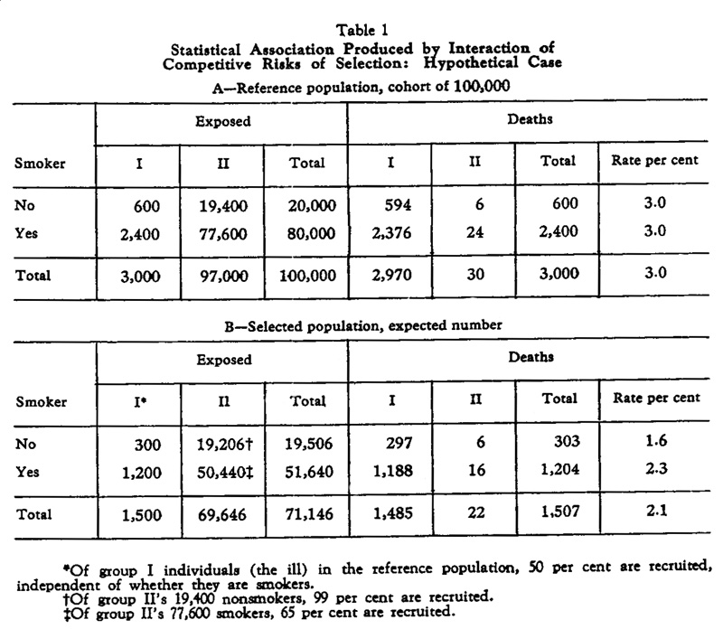
Note that the relative risk in the population is 1 but in the study population it is 2.3/1.6 = 1.438 or a 44 percent increase in deaths due to smoking.
This example was discussed in more detail in "The Nature of Statistics" by WA Wallis and JV Roberts. You can read their discussiion here.
REFERENCES
(1) James E. Enstrom and Geoffrey C. Kabat. Environmental tobacco smoke and tobacco related mortality in a prospective study of Californians, 1960-98. British Medical Journal. May 17, 2003 325:1057-1061.
(2) Jiang He, et al. Meta-analysis of epidemiologic studies. New England Journal of Medicine. March 25, 1999, 340:920-926.
(3). Kawachi I, et al. A prospective study of passive smoking and coronary heart disease. Circulation 1997;95;2374-9.
(4) Douglas G Altman, et al. odds-ratios should be avoided when events are common," BMJ 1998; 317: 1318.
(5) Mario Ciruzzi, et al. Case-control study of passive smoking at home and risk of acute myocardial infarction. Journal of the American College of Cardiology, March 15,1998:797-803.
(6) John C. Bailar III. Passive Smoking, Coronary Heart Disease, and Meta-Analysis. New England Joural of Medicine, March 25, 1999, 340:958-959.
(7) James E. Enstrom, Clarke W. Heath Jr. Smoking cessation and mortality trends among 118,000 Californians, 1960-97, Epidemiology 1999; 10:500-12.
(8) LeVois ME, Layard MW. Publication bias in the environmental tobacco smoke/coronary heart disease epidemiologic literature. Regul Toxicol Pharmacol 1995;21:184-191.
(9) Kyle Steenland, et al. Environmental tobacco smoke and coronary heart disease in the American Cancer Society CPS-II Cohort. Circulation 1996, 94:622-628.
This article is a good example of how a science writer, writing about a recent technical paper, can attempt to grab the attention of the reader. In the first paragraph we read:
Japanese, English, Swahili and Hungarian might sound completely unrelated, but it turns out that they have more in common than most of us realize. Researchers have identified a pattern in all human languages, and it now appears that this pattern may explain the very origins of how we began to talk.
Despite the somewhat exaggerated claim this is an interesting article. It will require that we refresh our memory about Zipf's law.
In 1916 the French stenographer J. B. Estoup (1) noted that if you listed words in a text according to the frequency of their occurrence, the product of frequency (F) and rank (R) of the words is approximately constant. Pereto (2) observed the same phenomena relating to corporate wealth. In his book "Human behavior and the Principle of Least Effort"(3) George Zipf showed that this constant product law applied to the ranking of populations of cities and had many more applications. This became known as Zipf's law.
At Keywordcount we were
able to obtain a frequency account just by providing the URL. Applying this
to the last issue of Chance News we looked for the top 20 words according to
frequency and checked Zipf's first law with the following table.
| Rank |
Word |
Frequency |
Rank x Frequency |
1 |
the |
466 |
466 |
2 |
and |
109 |
218 |
3 |
that |
99 |
297 |
4 |
for |
71 |
284 |
5 |
you |
68 |
340 |
6 |
this |
65 |
390 |
7 |
are |
61 |
427 |
8 |
from |
39 |
312 |
9 |
more |
35 |
315 |
10 |
with |
34 |
340 |
11 |
they |
31 |
341 |
12 |
medicare |
31 |
372 |
13 |
not |
31 |
403 |
14 |
have |
28 |
392 |
15 |
would |
26 |
390 |
16 |
was |
24 |
384 |
17 |
which |
24 |
408 |
18 |
chance |
24 |
432 |
19 |
will |
22 |
418 |
20 |
2003 |
22 |
440 |
Like most texts "the" and "and" have the highest frequencies and so have rank 1 and 2 respectively. Since these are small text we do not expect the products to be exactly equal but they are not too different. So Zipf's frequency law is suggested by even this small text.
To check this for a larger source we used the British National Corpus (BNC) mentioned in the last Chance News. This data set was described as follows:
The British National Corpus (BNC) is a 100 million word collection of samples of written and spoken language from a wide range of sources, designed to represent a wide cross-section of current British English, both spoken and written.
If product of rank and frequence is a constant then their log-log plot should be a straight line with slope -1. Here is a log-log plot of rank vs frequency for the BNC text:
![]()
The line with slope -1 fits the higher part of the graph corresponding to the most common words. But to fit the lower part of the graph (corresponding to words used infrequently) we had to choose a line with larger negative slope (1.64). The need for different lines for the frequent and the infrequent words was suggested by Ferrer-i-Cancho and Solé in their paper "Two regimes in the frequency of words and the origins of complex lexicons" (4). These authors also illustrate Zipf's laws as applied to the British National Corpus data.
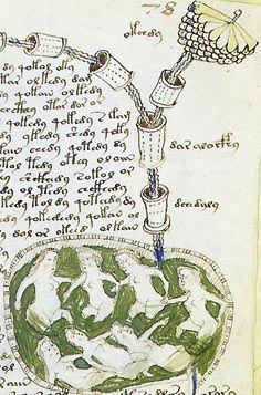
Here is an interesting application of Zipf's law carried out by Gabriel Landini. The Voynich manuscript is a famous manuscript shrouded in mystery. This mystery is described by Victory Segal in her brief account of a BBC4 documentary in the Sunday Times (London) 8 Dec. 2002. She writes:
While it is easy to mock conspiracy theorists as loners in X Files T-shirts, this documentary explores a puzzle whose appeal stretches way beyond the glow of the internet chat room. The Voynich manuscript was discovered in an Italian villa by an antiquarian book dealer, Wilfred Voynich, early last century. Decorated with pictures of plants, stars and "naked nymphs", its 238 pages are written in an unreadable language, a peculiar grid of symbols that have resisted all attempts at translation.
Some think it is a code, others a language in its own right. It might come from the 13th century or it might be a modern forgery, perpetrated by Voynich himself. This is a perfect introduction to the manuscript and its lore, veering between theories at a dizzying rate. Roger Bacon, John Dee and Emperor Rudolph II all play their part, as do National Security Council cryptographers, Yale maths professors and an array of eccentric amateurs, from computer games programmers to herbalists. And, of course, there is a man in South Carolina who thinks extraterrestrials hold the key.
You can find more details of the history and and current research on the web. We enjoyed the discussion here which has several nice pictures from the manuscript including this one:
Several electronic versions of the Voynich manuscript which use arbitrary alphabets to transcribe the symbols are available. These have been used to study statistical properties of the manuscript. In particular, Landini used two of these to see if Zipf's law applied to the frequencies of the Voynich text. His results are described here. Here are plots that he gives for the Rank-Frenquency relation using a translation called vornich.now:
For comparison Landini gives similar plots for several well known text sources including Alice in Wonderland:
Of course it would be nice if one could conclude that the Voynich manuscript is not a hoax from the fact that the frequency of words in the Voynich manuscript satisfy Zipf's law. This is complicated by the fact that it has been verified, by a number of studies that words generated randomly also appear to satisfy Zipf's law. However, a non-random hoax would probably not satisfy Zipf's law.
Zipf did not give a mathematical formulation but, as the title of his book suggests, he had the idea that it was related to a principle of least effort. For the case of development of a language Zipf wrote:
Whenever a person uses words to convey meanings he will automatically try to get his ideas across most efficiently by seeking a balance between the economy of a small wieldy vocabulary of more general reference on the one hand, and the economy of a larger one of more precise reference on the other hand, with the result that the vocabulary of different words in his resulting flow of speech will represent a vocabulary balance between our theoretical Forces of Unification and Diversification.
In their paper "Least effort and the origins of scaling in human language," Ferrer-i-Cancho and Solé provide a simple mathematical model which supports the idea that human language develops in such a way as to balance the effort of the speaker and the listener.
The authors represent a language with m words to describe n objects as an m by n matrix A= (aij) of 0's and 1's with aij = 1 if the ith word refers to the jth object. For example, suppose there are only four objects and these are described by four words with A given by:
o1 |
o2 |
o3 |
o4 |
|
|
w1 |
1 |
1 |
||
|
w2 |
1 |
1 |
||
|
w3 |
1 |
|||
|
w4 |
1 |
1 |
Note that words w1and w4 have two different meanings and object o1 can be referred to by two different words. The authors assume that there is at least one word referring to each object and, if the speaker has more than one choice, he makes a random choice. Finally, they assume that the objects occur with equal probabilities. Let p(wj) be the probability that the speakers will use word wj. Then in our example if 01 occurs (probability 1/4) the speaker uses w1 with probability 1/2. And if 04 occurs (probability 1/4) the speaker is sure to use w1. Hence p(w1) = 1/8 + 1/4 = 3/8. Similar calculations gives p(w2) = 1/4, p(w3) = 1/8, and p(w4) = 1/4.
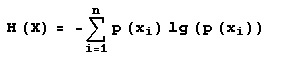
Now we can consider the object chosen as a random variable O with distribution p(oj) and the word chosen to represent this object as another random variable W with distribution p(wi). The authors call, what we call words, signals and use S am R for these random variables. To measure "effort" the authors use Shannon's entropy so we need to review a few definitions from information theory. You can find more about these quantities at Miachael Sosse's website.
Let X and Y be random variables with discrete distributions p(x) and p(y). Then the "entropy" of X is:
The "conditional entropy given Y = y" is :
![]()
And the "conditional entropy given Y" is
![]()
Finally, the "mutual information" of X and Y is:
![]()
The authors define the "effort of the speaker" to be the entropy Hn(W) where the subscript means the logarithms are computed to the base n. This is minimum when the same word is used no matter what the object.
They define the effort of the listener to be Hm(W|O). The effort for the listener is minimum when each word describes a unique object.
They define the cost function W(l ) as a mixture of the efforts for the listener and the speaker:
W(l ) = l Hn(W) + (1-l )Hm(W|O)
The authors then ask, for given values of l, m, and n, how do we find an m by n matrix A( l) of 0's and 1's that minimizes the cost W(l )? For this they use the following algorithm.
Starting from a given word-object matrix A, the algorithm performs a change in a small number of bits (specifically, with probability n , each aij can flip). The cost function is then evaluated, and the new matrix is accepted provided that a lower cost is achieved. Otherwise, we start again with the original matrix. At the beginning, A is set up with a fixed density of ones. This process is continued until there has been a specified time T without improvement.
The authors carry this out to determine the mimimum effort matrices A( l) for values of l from 0 to 1. They then plot the mutual information of W given O and the effective size of the alphabet as a function of l. The effective vocabulary of the matix is the number of words that refer to at least one object i.e. the number of non-zero rows in A( l). The results are shown in the following pair of graphs. The graph on the left is the plot ofthe multual information I(W|O) as a function of l and the graph on the right is a plot of the effective vocabulary L as a function of l.
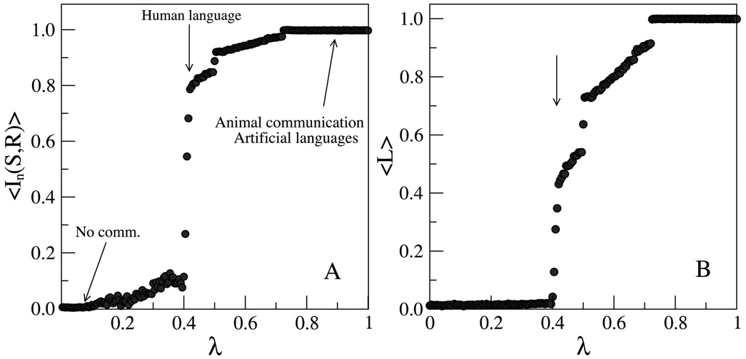
We see in these pictures that there appears to be a "phase transition" which the authors estimate to be about l* =4.1.
According to Zipf's law the log-log plot of k versus p(k) should be approximately a line with slope -1. To test this, the authors made log-log plots of k versus p(k) for different values of k. They obtained the following results for (a) l = .3 , (b) l* = .41 and (c) l = .5
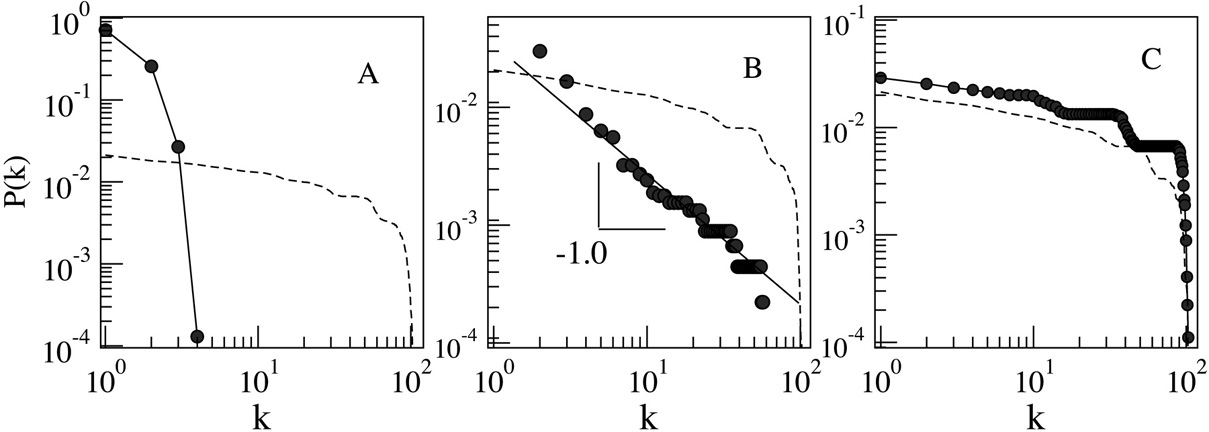
The plot for the critical value l* fits the Zipf's law prediction but neither of the other two do. The dotted lines show the distribution that would be obtained if the words and objects connected after a Poissonian distribution of degrees with the same number of connections of the minimum energy configurations.
Thus the authors have a model which supports Zipf's idea that his law results from a balanced effort required from the speaker and the listener.
This is a fun model to experiment with, but this is not for a Sunday afternoon at your computer. The authors program to carry out the algorithm to find minimum cost matrices was written by Ferrer-i-Cancho who is a computer scientist. To get the results shown in the last graphic the authors used matrices of size 150 by 150 and, for their algorithm to determine the minimum cost matrix, required a very small probability of changing an entry (0.0000447) and the number of repetitions with no improvement required to stop was very large (45,000). Then to avoid sampling variations the authors averaged 30 replications every time a minimum cost matrix was computed.
Ferrer-i-Cancho writes "The calculations in our paper took 3 weeks on a P IV at 2.4 Ghz (my calculations were the only program running)."
However, with a lot of help from Ferrer-i-Cancho and from our friendly programmer Peter Kostelec, we wrote a program that allowed us to make the required computations for 30*30 matrices and we did get results consistent with those demonstrated in the last two graphics.
References:
(1) J. B. Estoup. Gammes Stenographiques. Institut Stenographique de France, Paris, 1916.
(2) V. Pareto. Cours d'economie politique (Droz, Geneva Switzerland, 1896) (Rouge, Lausanne et Paris), 1897.
(3) G.K. Zipf. The Principle of Least Effort: An introduction to Human Ecology. Addison-Wesley, 1949
(4) Ferrer-i-Cancho, R. and Solé, R. V. (2001). Two regimes in the frequency of words and the origins of complex lexicons: Zipf's law revisited. Journal of Quantitative Linguistics, 8(3):165--173.
(5) Ferrer-i-Cancho, R. and Solé, R. V. Least effort and the origins of scaling in human language. Proceedings of the National Academy of Sciences. Feb. 4, 2003,788-791.
Copyright (c) 2003 Laurie Snell
This work is freely redistributable under the terms of the GNU General Public License published by the Free Software Foundation. This work comes with ABSOLUTELY NO WARRANTY.