Prepared by J. Laurie Snell, Bill Peterson, Jeanne Albert, and Charles Grinstead, with help from Fuxing Hou and Joan Snell.
We are now using a listserv to send out Chance News. You can sign on or off or change your address at this Chance listserv. This listserv is used only for mailing and not for comments on Chance News. We do appreciate comments and suggestions for new articles. Please send these to:
jlsnell@dartmouth.edu
The current and previous issues of Chance News and other materials for teaching a Chance course are available from the Chance web site.
Chance News is distributed under the GNU General Public License (so-called 'copyleft'). See the end of the newsletter for details.
Ranges are for cattle; give me a number!
President Lyndon Johnson
Contents of Chance News 10.11
1. Forsooth.
2. A Ripley Forsooth.
3. Fifth grade students to see Harry Potter movie an average
of 100,050,593 more times.
4. Bamboozled by statistics.
5. Is a record warm November evidence of global warming?
6. Study suggests that Lou Gehrig's disease is associated with
service in the Gulf War.
7. What Stanley H. Kaplan taught us about the SAT.
8. Richardson's statistics of war.
9. Shotgun wedding magic.
10. The newspapers' recount suggests that the Supreme Court did
not determine the winner.
11. A statistical argument that the 17th Earl of Oxford authored
the works of Shakespeare.
12. Chance Magazine has a new editor.
13. Are there boy or girl streaks in families?
14. We return to Lewis Carroll's pillow problem.
Migraines affect approximately 14% of women and 7% of men; that's one fifth of the population.
Herbal Health Newsletter Issue 1
undated
Nine out of ten people said that health was the most important issue in the election; four out of ten said Europe was the most important issue.
BBC Radio 5 Breakfast Programme
29 May 2001
Between 1974 and the end of 2000 the [pulp and paper] industry underperformed the overall European market by a shocking 914%
The Economist
15 September 2001
A reader,whose name we have regrettably lost, suggested a Forsooth item from a Ripley's Believe it or Not cartoon. According to the November 16th 2001 cartoon:
Jacob Ryan Slezak of La Jolla, Calif. was born on December 9, the same day as his mother, Colette, and his grandmother, Ellen Pourian were born! The odds of this happening are 48,627,125 to 1!
(1) How were the odds of 48,627,125 to 1 determined?
(2) Estimate the number of people in the U.S. that "Believe it or Not" could have chosen for its cartoon?
"Real critics," of course, refers to the kids who couldn't get enough of the Harry Potter movie, not the professional reviewers who panned it as "sugary and overstuffed."
The article reports that: "On average, the fifth graders Newsweek talked to wanted to see it 100,050,593 more times each. (Not counting those who said they'd see it more than 10 times, the average dropped to a reasonable three.)"
DISCUSSION QUESTION:
What can you say about the data based on these summaries? Is it possible to make an educated guess about the size of the sample or the magnitude of the outliers?
Giles wonders why, with all the improvements in gathering data and advances in statistics, we are still misled by numbers. He remarks that Darrll Huff's classic book, "How to Lie with Statistics" is as relevant as it was 40 years ago when it was written. In particular, he feels that more intelligent use of statistics should be used in political policy decisions and mentions the following example.
US studies have shown that men with low income and little education are twice as likely to suffer from strokes and lung disease and have a higher risk of dying early. In making decisions about redistributing money on healthcare for the elderly poor, the government needs to know whether being poor leads to worse access to the healthcare system or whether a bad health history tends to impoverish people.
Giles writes:
Speaking at a recent conference to promote the development, understanding and application of modern statistical methods, Nobel prize winner Danniel McFadden said that by analyzing people over time he could show that, in general, the link between low socio-economic status and death was not causal. Historic factors caused premature death among the poor, not falling down the socio-economic table.
McFadden's remarks are based on work reported in the paper "Healthy, Wealthy, and Wise?" co-authored with M Hurd, A. Merrill, and T. Ribeiro to appear in the Journal of Econometrics. You can read this paper here.
Giles goes on to say:
This sort of meticulous research should be at the centre of public policy debates and drive business decisions. But it rarely does. What is to blame? Three things: the frequency with which data are abused by people with a motive; our own tendency to dismiss good statistics as well as bad; and the statistical profession, for failing to communicate advances.
Evidently McFadden told the following story in his talk: When he was on the Council of Economic Advisers in 1964 and President Lyndon Johnson was presented with a range of forecasts for economic growth President Johnson replied:
Ranges are for cattle; give me a number.
Daniel McFadden was awarded his Nobel prize for developing statistical analysis that could be applied to discrete choices people face in their everyday lives. You can view McFadden's Nobel lecture on his work here.
Why do you think politicians don't make better use of statistics?
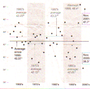
As its headline suggests, temperatures this fall have been unusually high. At 47.7 degrees Fahrenheit, the average November temperature for the United States was the second highest on record; the average since 1895 is 42.6 degrees. Scientists have proposed several possible contributing factors, such as the Madden-Julian Oscillation, a roughly 50-day cycle of hot and cold temperatures in the Western Pacific that has been in its hot phase this fall. Another theory cites this fall's unusually strong zone of high pressure over the Azores that has prevented the jet stream from following the more typical path which is closer to the Northeastern U.S. But a complete understanding of the processes that produce temperature fluctuations is as yet elusive.
Indeed, even determining what is meant by the phrase "warming trend" can be problematic. According to the article, weather experts caution against viewing this fall's higher temperatures as part of "the long-term phenomenon of global warming." Dr. Matthew A. Barlow of Columbia University's International Research Institute for Climate Prediction says that "it's very difficult to separate when you're just getting a run of events versus something responding to a longer signal." He adds, "Weather is often like flipping a coin. You're bound to get five heads in a row sometimes."
The article includes the following nice graph to show the variation in the average November temperatures over recent years.
Last month was the second warmest November on record in the United Sates, but the previous November was the second-coldest. Dots represent annual November temperature average. Source: Pennsylvania State University, Meterorology Department, The New York Times
(1) What do you think Dr. Barlow means by the statement "weather is often like flipping a coin."? Why do you think he said, "You're bound to get five heads in a row sometimes." ?
(2) The article states that "the recent weather is simple a matter of 'the noise' of natural variability, more of which is on the way..." What do you think this means? What might "unnatural variability" be? How might you measure it?
After years of denying that they could find a link between illness and service in the Gulf War, a joint announcement by the Defense and Veterans Affairs Departments said that they would immediately offer disability and survivor benefits to affected patients and families. This announcement was in response to a study conducted at a veterans hospital in Durham, N.C. that found that veterans of the Gulf War were twice as likely as other soldiers to suffer the fatal neurological disease called Lou Gehrig's disease.
The study identified 700,000 soldiers sent to the Gulf from August 1990 to July 1991 and 1.8 million other soldiers who were not in the Gulf during this time period. It was found that, during this period, 40 of the 700,000 Gulf War veterans had been diagnosed with Lou Gehrig's disease and 67 of the 1.8 million other soldiers had developed this disease. The Times article states:
The authors did not offer theories on why Gulf War veterans would be at increased risk. Nor did they say what the odds were that the finding occurred by chance... . The study has been submitted for publication in an academic journal.
It is not hard to estimate the odds. There were 107 people identified with Lou Gehrig's disease among the population of 2.5 million people. If there was an association with the Gulf War the number from the Gulf group could be modeled by the number of heads when a coin with probability p = 7/25 for heads is tossed n = 107 times. The probability of getting 40 or more heads when such a coin is toss is .022. Thus, if we consider a one-sided test, the result is significant at the 5% level. If we consider a two-sided test it would still be significant but just barely.
An editorial in the NYTimes (16 Dec. 2001, section 4 page 12) related to this study comments:
The chief question that will need to be addressed by peer reviewers is whether the study was able to ferret out cases of Lou Gehrig's disease with equal success in both groups, namely those who served in the Gulf and those who did not. With all the uproar in recent years about illnesses found among Gulf War veterans, it seems likely that the researchers identified everybody with Lou Gehrig's disease in that group. The issue will be whether the study, through advertising and contacting patients' groups and doctors, was able to find virtually all the cases in the other group as well. If they missed some, the difference between the two groups might disappear, and service in the Gulf would not be associated with risk of the disease.
In fact if the researchers found all those who were diagnosed with Lou Gehrig's disease in the Gulf group but missed six or more in the larger control group even the one-sided test would no longer be significant.
(1) Do the results of this study seem convincing to you?
(2) Do you think the government was justified in not waiting for the results to be peer reviewed?
(3) The article stated that among Gulf War veterans, the risk of disease was 6.7 cases per million over a ten-year period. Among other military personnel, it was 3.5 per million over this same period. On the basis of these numbers the article stated that veterans of the conflict were nearly twice as likely as other soldiers to suffer the fatal Lou Gehrig disease. How did they arrive at these numbers?
This article, ostensibly a review of Kaplan's memoir, "Test Pilot", covers a lot of ground. In addition to an entertaining account of Kaplan's youth, the humble beginnings of his now ubiquitous test-preparation company, and the methods Kaplan developed for "beating" standardized tests, the article contains a concise summary of the reasons behind the University of California's recent proposal to discontinue using the SAT scores in admission decisions. The subtitle of Kaplan's book is "How I Broke testing Barriers for Millions of Students and Caused a Sonic Boom in the Business of Education". According to Gladwell, "that actually understates his importance. Stanley Kaplan changed the rules of the game."
The basis for Gladwell's remark is, in part, the fact that Kaplan refused to accept the persistent assertions by the E.T.S. and the College Board that the SAT cannot be coached. Such assertions of course support the notion that the SAT--especially the SAT I--is an objective measure of "innate" aptitude and therefore provides a more "objective" balance to high school grade point averages. For this reason, and several sordid others (also touched upon in the article), colleges and universities happily turned to the SAT to help them decide which students to admit. If, however, the SAT does not measure "innate aptitude" (whatever that might mean) then students should be able to improve their scores if they understand the underlying logic of the test and its makers. This assumption has apparently been the key to Kaplan's success.
The section of the article that describes UC's recent proposal to drop the SAT I begins ominously: "The SAT is seventy-five years old, and it is in trouble." Gladwell proceeds to summarize some of the results in the report "UC and the SAT: Predictive Validity and Differential Impact of the SAT I and SAT II at the University of California" (by Saul Geiser with Roger Studley, October 29, 2001. The report and data relating to the study are available here. The main conclusions of the study (which is highly readable) are:
(1) Among high school grade-point averages (gpa), SAT I scores, and SAT II scores, SAT II scores are the best predictor of freshman grades.
(2) SAT I scores explain only an additional .1% of variance over the 22.2% explained by HS gpa and the SAT II.
(3) When HS gpa is held constant (at the mean), the SAT II has about three times the predictive power of the SAT I: each 100-point increase in SAT II scores adds about .18 of a grade to freshman gpa compared to .05 for the SAT I.
(4) The SAT I is more sensitive to socioeconomic factors. Holding the log of family income and years of parents' education constant along with HS gpa yields about a .19 increase in freshman gpa for every 100-point increase in the SAT II compared to only a .019 increase for the SAT I.
The UC report also examines differences in performance on the tests between underrepresented groups, and discusses the potential impact on these groups of removing the SAT I from admissions decisions.
(1) Do you think the SAT should be used in making admissions decisions? Why or why not?
(2) The UC analysis does not include students who failed to complete their freshman year. Comment.
(3) Included in the UC report is a table that indicates, for given HS gpa's,
the minimum SAT I score necessary (prior to fall '01) to be eligible for
admission. Not surprisingly there is an inverse relationship up to a gpa of 3.3
and above, at which point any SAT I score is acceptable. (The SAT II scores are
apparently used to determine campus eligibility.) How might such a scheme affect
attempts to measure the relative predictive ability of the SAT I and HS gpa for
freshman grades?
Lewis Fry Richardson (1881-1950) was a pioneer in applied mathematics. For
example, he was the first to apply mathematical methods to weather predictions.
A fascinating account of Richardson's life and his work on weather predictions
is the subject of a previous Brian Hayes' Computing Science column titled The
Weatherman (American Scientist, January-February 2001).
In this
column, Hayes tells the story of Richardson's statistical analysis of wars.
Richardson tried to understand war by building and analyzing a database of some
315 conflicts from 1820 to 1950. One surprise was the essential randomness of
war as evidenced by the goodness of fit of a Poisson model to the incidence of
war.
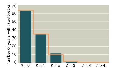
Frequency of outbreaks of war (blue bars) is very closely
modeled by the Poisson distribution (orange line), suggesting that the onset of
war is an essentially random process. (American Scientist January-February
2001).
Another was the huge impact of the two magnitude-7 world wars: they account for about sixty percent of all deaths. The magnitude of a war, as defined by Lewis Fry Richardson, is the base-10 logarithm of the number of deaths.The next most lethal group was a cluster of seven magnitude-6 conflicts, one of which was the U.S. Civil War, while most CMJ readers would likely have great difficulty naming any of the other six! (The seven are listed at the end of this Chance News)
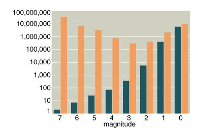
Magnitude of a war, as defined by Lewis Fry Richardson, is the base-10 logarithm of the number of deaths. Blue bars indicate the number of wars between 1820 and 1950 that are in each magnitude range; orange bars are the total deaths from wars of that magnitude. Two magnitude-7 wars account for 60 percent of all deaths.(American Scientist January-February 2001)
Having found no temporal explanations for war, Richardson turned to the question of whether wars tended to be between neighboring states. He found that smaller wars involving only two countries tended to be between neighbors. However he concluded that "chaos" was still the predominant factor in explaining the world's larger wars.
Finally, Richardson considered other causative factors such as social, economic, and cultural. He looked for correlation between these factors and belligerence. To his great dissapointment Richardson found essentially no correlation for these factors with the possible exception of religion. Hayes writes:
The one social factor that does have some detectable correlation with war is religion. In the Richardson data set, nations that differ in religion are more likely to fight than those that share the same religion. Moreover, some sects seem generally to be more bellicose (Christian nations participated in a disproportionate number of conflicts). But these effects are not large.
(1) How many of the seven magnitude-6 wars that Richardson identified between 1820 and 1950 can you list? (Richardson's seven are listed at the end of this Chance News.)
(2) A more up-to-data data base on wars can be found at the Correlates of War web site. See if you can determine, from the data available from this web site, if Richardson's conclusions are still valid.
Writing about Richardson's geographic study of the smaller wars between two countries Hayes says:
During the period covered by Richardsonís study there were about 60 stable nations and empires (the empires being counted for this purpose as single entities). The mean number of neighbors for these states was about six (and Richardson offered an elegant geometric argument, based on Eulerís relation among the vertices, edges and faces of a polyhedron, that the number must be approximately six, for any plausible arrangement of nations). Hence if warring nations were to choose their foes entirely at random, there would be about a 10 percent chance that any pair of belligerents would turn out to be neighbors. The actual proportion of warring neighbors is far higher. Of 94 international wars with just two participants, Richardson found only 12 cases in which the two combatants had no shared boundary, suggesting that war is mostly a neighborhood affair.
What is Euler's relation and how do you think Richardson used it to show that the mean number of neighbors of a nation must be about six?
Observational data suggest that married men enjoy an earnings advantage--variously estimated at 10 to 20 percent--over single men with similar age, education and job type. Some investigators have explained this "marriage premium" by noting that the same personality and intelligence traits that make a man valuable to employers may also make him attractive to potential spouses.
A recent study in the "Journal of Population Economics" looked at the problem from a provocative angle, breaking out the data for men whose first child was born within seven months of the wedding. Since some of these marriages may have been hastily entered because of the pregnancies, the explanation given above for the earnings effect might not hold up. The researchers therefore compared this group of men to those whose first children came later in their marriages. However, after controlling for other relevant variables, they concluded that "about 90% of the marriage premium remains."
The new study estimates the overall marriage premium as 16 percent. The researchers explained that getting married may lead men to focus more on earning. They added that other investigators believe that employers may actually be discriminating against single men.
(1) Can you think of any other explanation for the "marriage premium." How might you test it?
(2) Do you think there is a marriage effect for women?
Each year, farmers in the Junagadh region of India face the choice of planting peanuts or castor. Peanuts thrive in wet conditions, while castor is more resistant to drought. But the crucial planting decisions have to be made in April or May, before the rains of the monsoon season arrive in June. In the absence of scientific forecasts, farmers have traditionally relied on folk wisdom.
For the last five years, Dr. P. Kanani of the Gujarat Agricultural University has been studying these folk methods. One predicts that the monsoon rains will begin 45 days after the full bloom of the C. fistula tree. A chart accompanying the article presents Dr. Kanani's data, showing that since 1996 the start of the monsoon season seems to follow the predictions, though there is somewhat more variability in the actual start dates than in the predictions. A second method considers the wind direction on the Hindu festival day called Honi, which occurs in the spring. In years which subsequently had average to above-average rainfall, the wind on Honi had come from the north or west; in below-average years, it had come from the east.
Professional weather forecasters pooh-pooh such methods. Still, it is not clear where the farmers should turn. In each of the last 13 years, India's director-general of meteorology has predicted a "normal" monsoon season. Indeed, the overall national averages for rainfall have been in the "normal" range. But this is little help to local farmers who need advice specific to their own regions. (This discussion reminded us of two lectures from our 1997 Chance Video series. Professor Daniel Wilks of Cornell University talked about mathematical models for national weather forecasting and Vermont forecaster Mark Breen described the challenges of providing advice to farmers about local variations.)
Meanwhile, Dr. Kanani hopes to develop a full-fledged research proposal on
the folk methods that will meet the standards of peer review.
A total of 175,010 ballots were disqualified during the 2000 election debacle in Florida. Included in these were "overvotes," where more than one presidential choice was indicated, and "undervotes," where no vote was registered by the voting machines. (In the latter category are the infamous punch card ballots with "dimpled" and "hanging" chads.) Beginning last December, a consortium of eight news organizations, which included USA Today and the New York Times, undertook a complete examination of all the disqualified ballots. This painstaking task has recently been concluded.
According to USA Today, the study found that ballot design played a larger role in disqualifying votes than did the voting machines themselves. Especially troublesome was the two-column format used in Palm Beach County and elsewhere, which gave rise to overvotes when people thought they needed to indicate choices for both president and vice president. Voting rights advocates have been calling for overhaul or replacement of antiquated voting machines; this is an expensive proposition, and the study suggests that it might not be the answer. The article states that old-fashioned punch card and modern optical scanning machines had "similar rates of error in head-to-head comparisons."
In addition to variations in ballot design and voting machines, the study considered demographic variables such as educational level, income, age and race in order to determine which factors may have contributed to votes being disqualified. Of course, the ballots themselves are secret. But because the new study was conducted at the precinct level--as compared with earlier analyses by counties--more detailed demographic inferences can be drawn.
Punch card ballots appear to have been a particular problem for older voters, who may have had trouble pushing hard enough to remove the chad and register a clean vote. Precincts whose populations had larger proportions of elderly voters had comparatively larger undervote rates.
Experts had more difficulty explaining the trends that emerged concerning race. Even after controlling for age and education, blacks were three to four times more likely than whites to have their ballots rejected. Professor Philip Klinkner, who teaches political science at Hamilton College, said that this "raises the issue about whether there's some way that the voting system is set up that discriminates against blacks." A surprising response was put forward by John Lott of the American Enterprise Institute, who argued that the highest rate of disqualification was experienced by black Republicans. You can read details of Lott's argument in the op-ed piece from the L.A. Times ("GOP was the real victim in Fla. vote," by John R. Lott and James K. Glassman, Los Angeles Times, 12 November 2001, Part 2, p. 11). You can find an account of Lott's research that was the basis of this article here.
The second New York Times article points out that even after a year of discussion, the latest study still has not produced a definitive statement of who actually got the most votes. If there is one reassuring finding, it is that the controversial Supreme Court ruling did not hand the election to Bush. If the manual recount of 43,000 votes initiated by Gore had been allowed to continue, it appears that Bush still would have prevailed. The present study considered an even larger set of disqualified votes; but, in the end, it found that the tally can go either way depending on the standards used to admit those ballots. The Times maintains a web page devoted to the Florida vote. An interactive feature there allows users to select from a number of available criteria for accepting ballots. You can try it yourself here.
More enterprising readers may wish to download the full data set for the study, which is available from the USA Today web here.
(1) What do you think USA Today means by a "head-to-head comparison" of punch-card vs. optical-scan voting machines?
(2) Lott's piece in the L.A. Times says that African American Republicans
were 50 times more likely than other African Americans to have their ballots
disqualified. He concludes that "if there was an concerted effort to prevent
votes from being counted in Florida, that effort was directed at Republicans,
not at African Americans." What do you make of this?
Our colleague David Web participates in a Shakespeare news group.From time to time David asks us about statistical arguments used in the controversy about the identity of Shakespeare. He asked us to comment on this appendix to a recent thesis by Stritmatter. In his thesis, Stritmatter studied a Bible owned by the 17th Earl of Oxford, Edward de Vere-- the leading candidate for those who believe that the name Shakespeare was a pseudonym for another author. The de Vere Bible had a large number of marked verses some of which were also used in the works of Shakespeare.
McGill's analysis is based on the following assumptions: There are about 30,000 verses contained in the New and Old Testament of which about 1 in 3 or 10,000 might yield a useable reference for an author. Stritmatter found 1083 marked verses in the de Vere Bible, and based on his and other experts research, about 982 unique Biblical verses used by Shakespeare. Strittmatter identified 199 verses that were both in Shakespeare's works and in the de Vere Bible. So McGill asks: could an overlap as large as this occur by chance?
To answer this, he assumes that the 1083 choices in the de Vere Bible represent a random sample chosen randomly without replacement from the set of 10,000 possible verses in the Bible. Then the distribution of the overlap with the the 982 verses used by Shakespeare would have a hypergeomtric distribution. The hypergeometric distributions has three parameters: the population size N = 10,000, the number of successes s = 982 (verses used by Shakespeare) and the sample size n = 1083 (versus in the de Vere Bible). Then if p = s/N and q = 1-p the expected size of the overlap is np = 104.4 and the variance = npq(N-n)/(N-1) = 84.14 giving a standard derivation of 9.17. The overlap of 199 is 95 greater than the expected number 104 which translates to about 11standard deviations greater. Such a difference could hardly occur by chance.
McGill remarks that if we reduce the estimate for the number of useable Bible verses or increase the number of the number that are used in Shakespeare's works it becomes harder to reject the chance explanation. For example if 1 in 4 of the Bible verses are usable and Shakespeare used 1200, then the mean is 170 which is only 2.3 standard deviations from the mean.
But even if McGill's assumptions are reasonable and the results are significant, one has to ask if the model McGill rejects is a reasonable null hypothesis for no association. For example, surely deVere would not choose verses at random to mark. In fact, his favorites might also be Shakespeare's favorites which would give a significant overlap even if de Vere is not Shakespeare.
(1) What do you think of McGill's argument?
(2) McGill comments that one should really use a Bayesian analysis since
researchers have given other arguments that the Earl of Oxford was Shakespeare.
You can find these at the Shakespeare Oxford Societyweb site
dedicated to showing that de Vere was Shakespeare. Based on these, we could
determine an apriori probability that Shakespeare was the Earl of Oxford. Then
we could compute the apostori probability based on the new evidence provided by
the de Vere Bible. Of course we would also have to use the arguments found at
the The Shakespeare Authorship
Page dedicated to the proposition that Shakespeare wrote Shakespeare. Do you
think that a Bayesian approach would help settle this argument?
This is the last issue of Hal Stern's term as Editor. Hal has been a fine editor and has attracted outstanding articles for Chance Magazine. This is particularly true of this current issue. You can see the highlights of this issue here.
Hal has been especially effective in obtaining articles on controversial
topics and having other experts give commentaries on these articles. In this
current issue, this is the case for an article "Misuses of statistics in the
study of intelligence: the case of Arthur Jensen" by Jack Kaplan. Commentators
are Conor Dolan and Arthur Jensen. During Hal's editorial term, the Chance
Magazine web site has been significantly improved and also now includes PDF
versions of previous issues, lead articles, highlights of previous issues, and
indexes.
The new editor is Dalen Stangle, Professor of the Practice of
Statistics and Public Policy, at the Institute for Statistics and Decision
Sciences of Duke University. We wish her success in this important
position.
As usual we will comment only on our own favorite article since
we assume that most of our readers subscribe to Chance Magazine. It happens that
our favorite article is also their featured article so you can find this article
here if
you do not get Chance Magazine (though you should).
There have been many studies involving large data sets in several different countries that attempted to see if the Bernoulli trials model can explain the distribution of boys and girls in a family. For a Bernoulli trials model the distribution of boys in a family of size n should have a binomial distribution with p about .51. Perhaps the largest study was carried out in Germany in 1889 by A. Geissler. This study involved some four million births. Geissler concluded that the Bernoulli trial model did not fit the data but he did not have a method to test the fit. R.A. Fisher, in his classic "Statistical Method for Research Workers" uses Geissler's data to illustrate the Chi-Square test. Fisher considered families of size 8 and provides the following table derived from Geissler's data.
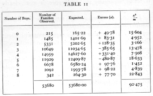
Using the Chi-Squared test we find that p is less than 0.0001 so we would reject the hypothesis that the distribution of the number of boys in a family is a binomial distribution. Fisher also notes that there are too many families with an even number of boys. As another test, Fisher shows that the variance of the distribution is significantly larger than would be expected by a binomial distribution. You can read his discussion of this example here (see section 18: "The Binomial Distribution")
The history of this problem can be found in an article by A.W.F. Edwards (Edwards, A.W.F.(1962), "Genetics and the human sex ratio," Advanced in Genetics, 11, 239-272). Edwards discusses the Geissler study and three other large studies: a Swedish study of 5,477 Swedish families, a French study of 14,230 French families of five or more children, and a Finnish study of 60,334 Finnish families. Another large study carried out after the Edwards article was a study by Greenwood and White (Greenberg, R. A, and White, C (1967), "The sexes of consecutive sibs in human sibships," Human Biology, 39, 374-404).This is a study with data consisting of 116,458 families collected from the archives of the Genealogical Society of the Church of Jesus Christ of Latter Day Saints at Salt Lake City, Utah.
The Swedish study concluded that the Bernoulli trials model did reasonably fit the data. The French study and the Finnish study both rejected this hypothesis finding a significant positive correlation between successive births. But as Edwards remarks, tests for a binomial distribution for families of a fixed size can be confounded by stopping rules. For example, in an extreme case, assume that families have children only until they have a girl. Then the distribution of families of size 1 would have 100% girls!. As another example, families may try to have a "balanced" family, i.e., a family with at least one boy and at least one girl. If so, when the first two children are BG or GB they might tend to stop having children but if they are BB or GG to have another child. This would result in fewer BB or GG sequences in families of size 2 than would be expected by the Bernoulli trials model. This problem could be resolved by looking at the distribution of the first child, the first two children, etc.
For this article Rodgers and Doughty obtain new data to do their own study of this problem. They use data obtained from the National Longitudinal Survey of Youth (NLSY). In 1979, over 12,000 respondents aged 14-21 were obtained from a probability sample of 8,770 households in the United States. This original sample has been followed since that time. By 1994 the respondents were aged 29-36 and most the of their childbearing was completed. The authors used this 1994 data. There were not many families with more than four children, so the authors restricted their study to families with at most four children. This resulted in a sample of 6,089 families. Throughout this discussion we always understand biological children.
The distribution of birth patterns in their sample is:
| pattern | frequency | proportion |
| B |
930 |
0.1527 |
| G |
951 |
0.1562 |
| BB |
582 |
0.0956 |
| BG |
666 |
0.1094 |
| GB |
666 |
0.1094 |
| GG |
530 |
0.0870 |
| BBB |
186 |
0.0305 |
| BBG |
177 |
0.0291 |
| BGB |
148 |
0.0243 |
| BGG |
173 |
0.0284 |
| GBG |
182 |
0.0299 |
| GBB |
151 |
0.0248 |
| GGB |
125 |
0.0205 |
| GGG |
159 |
0.0261 |
| BBBB |
43 |
0.0071 |
| BBGB |
26 |
0.0043 |
| BGBB |
30 |
0.0049 |
| BGGB |
23 |
0.0038 |
| GBGB |
23 |
0.0038 |
| GBBB |
32 |
0.0053 |
| GGBB |
29 |
0.0048 |
| GGGB |
29 |
0.0048 |
| BBBG |
34 |
0.0056 |
| BBGG |
37 |
0.0061 |
| BGBG |
22 |
0.0036 |
| BGGG |
24 |
0.0039 |
| GBGG |
28 |
0.0046 |
| GBBG |
29 |
0.0048 |
| GGBG |
28 |
0.0046 |
| GGGG |
26 |
.0043 |
| total |
6089 |
1 |
From this table we find that the 6089 families had a total 6389 boys and 6135 girls resulting in a proportion of boys of .510.
We note that in families of size 1 there were more girls than boys. This could be explained by chance or by a tendancy for families to stop having children when they have a girl. Looking at families with two children we see
| BB |
582 |
| BG |
666 |
| GB |
666 |
| GG |
530 |
so there are more BG and GB than BB and GG. This could caused by chance but also by a preference for "balance" families. As we have remarked, the effect of a stopping problem will be removed if we look at the patterns for the first child, the first two children etc. . Here are the results up to the first three children.
|
Pattern |
frequencies | expected |
|
First child |
||
|
B |
3101 |
3105.4 |
|
G |
2988 |
2983.6 |
| total |
6089 |
6089 |
|
First two children |
||
|
BB |
1085 |
1094.5 |
|
BG |
1086 |
1051.6 |
|
GB |
1111 |
1051.6 |
| GG |
926 |
1010.3 |
|
total |
4208 |
4208 |
|
First three children |
||
|
BBB |
263 |
234 |
|
BBG |
240 |
224.8 |
|
BGB |
200 |
224.8 |
|
GBB |
212 |
224.8 |
|
BGG |
220 |
216 |
|
GBG |
233 |
216 |
|
GGB |
182 |
216 |
| GGG |
214 |
207.5 |
|
total |
1764 |
1763.9 |
Now, for the first child, the proportion of boys is 3130/6089 =.509 is very close to the population proportion of .51. Looking at the first two children we see that the balance effect has disappeared but we appear to have too few GG families. A Chi-Squared test on the first two children would reject the Bernoulli model with p = .01. The Bernoulli trials fit for three children looks pretty good except for the GGB pattern. This is probably caused by the smaller number of GG families in the first two children. For first three children the Chi-Squared test would reject the Bernoulli trials model with p = .04.
This result is typical of the other studies. It is often easy to reject the Bernoulli trials model but very difficult to explain why this happens. Previous studies have suggested the following possible explanations for the deviation from the simple Bernoulli model.
(a). There is a correlation between the sex of successive children (the subject of this article).
(b) The probability of a boy differs between families. For example, it has been documented that different races have different sex ratios. See for example (Erickson, J. D. (1976), "The secondary sex-ratios in the United States 1969-71," Annals of Human Genetices 40, 205-212).
(c) the probability of a boy varies within a family,
(d) the birth order is affected by a couple's stopping preferences.
Methods to sort out these possibilities were presented in the study previously mentioned by Greenberg and White. H.H.Ku gave another approach to their method (Ku, H.H., (1971), "Analysis of Information -- An alternative approach to the detection of a correlation between the sexes of adjacent sibs in human families," Biometrics 27, 175-82,175-182). A completely different approach was developed by Crouchley and Pickles (Crouchley. R, and Pickles, A.R. (1984) Methods for the identification of Lexian, Poisson and Markovian variations in the secondary sex ratio, Biometrics 40, 165-175).
We will describe the method of Crouchley and Pickles since it is similar to that used by Rodgers and Doughty.
Crouchley and Pickles model the sex of successive children in a
family modeled by a non-stationary Markov Chain with a stopping rule T.
(Non-stationary means that the transition probabilities can change for
successive trials.) A decision to stop at time T is allowed to depend on the sex
pattern up to time T but not on future times, i.e., no extra sensory perception.
If the stopping time does not depend on the sex of previous children, we call it
a "constant stopping time." When the transition probabilities are the same for
each child we have a simple Markov chain with only one transition matrix needed.
If the probabilities for a boy or girl do not depend on the sex or the number of
previous children we have the Bernoulli trials model.
The probability that the first child is a boy, the transitions probabilities for the Markov Chain and the stopping rules provide the parameters for the model. To take into account the possibility of variation between families, mixing distributions for the transition probabilities are needed and will introduce additional parameters.
For a given data set, the parameters are chosen to maximize the log-likelihood function. The goodness of the fit is measured by a Chi-Squared test. Crouchly and Pickels applied this method to the data from the Finnish study and the Utah genealogical study. Before looking at the full model the authors consider special cases. For the Uath data they first obtain the best fit for a Bernoulli trials model with fixed stopping time. This resulted in a Chi-Squared value of 100.46 with 54 degrees of freedom (p = 0.000127 ). Allowing stopping time to depend on the previous sex pattern gave a Chi Square value of 23.02 with 29 degrees of freedom (p = 0.78) suggesting that the Bernoulli model with variable stopping rules described the data satisfactorily. In fact, the full model did not fit as well as the Bernoulli model.
Rodgers and Doughty follow a similar procedure but restrict their models to stationary Markov chains with stopping variables. They limit the stopping rules to those designed to test specific behaviors such as the preference for a balanced family. The best fit was determined by the parameters that gave the smallest Chi-Squared value. Rodgers and Doughty found that the best fit was a Bernoulli trials model with stopping parameters consistent with a desire for a balanced family.
Rodgers and Doughty also consider another interesting question related to the sex ratio, namely, is there a genetic effect on the sex ratio? The NSLSY dataset includes information necessary to create genetic links between biologically related respondents. This allowed the authors to test for a genetic effect on the sex ratio. For about 90% of the kinship pairs in the sample, the authors were able to identify a kinship pair as cousins, half siblings, full siblings, DZ twins or MZ twins. They carried out two correlation analyses. In both of these, the independent variable was a measure of the relatedness of the NLSY respondents. In the first correlation, the dependent variable was the proportion of the respondents' children who were boys and in the second correlation the dependent variable was the sex of the first child. Here are the results of their correlation computations.
Kinship Correlations
| Relation | Proportion of boys | First Child |
|
Cousins |
.35 (33) |
.21 (33) |
|
Half siblings |
.18 (98) |
.12(98) |
|
Full siblings |
.08(1129 |
.11(1131) |
|
DZ twins |
-.03(15) |
-.11(15) |
|
MZ twins |
-.20(6) |
-.03(6) |
Note: Sample sizes giving in parentheses
If there were a genetic or shared environment effect we would expect the correlations to increase as the level of relationship increases but, in fact it decreases. Thus the authors conclude that they cannot identify any genetic or shared environment effect.
So Joseph Rodgers concludes from this study that he has found no evidence that sex bias runs in the family despite the remarkable performance of the Rodgers men. He is consoled by the fact that since the time of his sister's pronouncement his brother and cousin have had three children, two daughters and one son. He has also contributed two girls so instead of 21 boys out of 24 children this generation of Rodgers men have produced a total of 22 out of 29 children. But it is still a pretty unlikely event since the probability of getting as many as 22 heads when you toss a coin 29 times is .004.
Ruma Falk informed us that, at the time they wrote their article, they were not aware of the following article on the same subject: Portnoy, S. (1994). "A Lewis Carroll pillow problem: Probability of an obtuse triangle," Statistical Science, 9(2), 279-284.
Portnoy discusses the general problem of defining randomness and illustrates his ideas in terms of the pillow problem.
In geometric probability problems there are two kinds of difficulties: (1) the problem asks us to choose numbers at random from an infinite set. This is not possible with the usual concept of randomness of making all outcomes equally likely (2) the problem can be solved, but the solution is not unique. The Lewis Carroll pillow problem to find the probability that a triangle chosen at random on the plane is obtuse is an example of both. It obviously has difficulty (1). Falk and Samuel-Cahn suggested avoiding this the problem by solving the problem on a finite region of the plane, say on a circle, and passing to the limit. However, as they show, if you do the same thing on a square you will get a different answer and a different limiting value. So, if we do this we have difficulty (2).
Another famous example of non-uniqueness is Bertrand's problem: Given a circle, find the probability that a chord chosen at random is longer than the side of an inscribed equilateral triangle. Here the problem is that you have to specify how the cord is determined and different ways of doing this give different answers. There is an excellent discussion of this problem on the Cut the Knot web site. Click here to see three different solutions which give the answers 1/4, 1/3, and 1/2. You will also find simulations to verify these answers.
E. T. Jaynes proposed the following way to determine a unique solution. Consider a real experiment involving throwing long straws at a circle drawn on a card table. A "correct" solution to the problem should not depend on where the circle lies on the card table, or where the card table sits in the room. Jaynes showed that if we required these two conditions we get a unique solution with the answer 1/3. His discussion of this approach can be found in "The Well-Posed Problem," in Papers on Probability, Statistics and Statistical Physics, R. D. Rosencrantz, ed. (Dordrecht: D. lReidel, 1983, pp. 133-148.).
Portnoy suggests the following solution to the pillow problem. A triangle is
determined by three points in the plane (x1,y1),(x2,y2),(x3,y3). Thus the set
of triangles in the plane can be identified with the six-dimensional space R^6.
He shows that if we choose a point in R^6 (and hence a triangle) by any spherically
symmtric probability measure on R^6 we will get the same value for the probability
that the resulting triangle is obtuse. Then by an argument similar to Jaynes,
Portnoy argues that any reasonable way to achieve choosing points at random
in the plane should have the property that the induced measure on R^6 is sperically
symmetric. Thus to solve the Pillow Problem we need find the probability that
a random triangle is obtuse for a particular spherically symmetric measure on
R^6. Portney does this by assuming that the the six coordinates are the outcome
of 6 independent normal random variables with mean 0 and standard deviation
1. For this spherically symmetric measure the probability that the resulting
triangle is obtuse is 3/4. So, this is Portnoy's answer to Lewis Carroll's Pillow
Problem.
The seven megadeath conflicts listed by Richardson are, in chronological
order, and using the names he adopted: the Taiping Rebellion (1851ñ1864), the
North American Civil War (1861ñ1865), the Great War in La Plata (1865ñ1870), the
sequel to the Bolshevik Revolution (1918ñ1920), the first Chinese-Communist War
(1927ñ1936), the Spanish Civil War (1936ñ1939) and the communal riots in the
Indian Peninsula (1946ñ1948).
Copyright (c) 2001
Laurie Snell
This work is freely
redistributable under the terms of the GNU
General Public License
published by the
Free Software Foundation.
This work comes with ABSOLUTELY NO
WARRANTY.