Prepared by J. Laurie Snell, Bill Peterson, Jeanne Albert, and Charles Grinstead, with help from Fuxing Hou and Joan Snell.

This will be our last issue of Chance News. The current authors of Chance News are planning to write some chapters on issues that have come up in previous issues of Chance News such as fingerprinting, streaks in sports, statistical tests used in medical studies etc. We will make these available on the chance website as they are written.

We hope that one of our readers will be interested in continuing Chance News. To encourage this we will put references to articles that would be appropriate for future chance news issues on the chance website under "current chance news articles." Please continue to send suggestions with comments or a complete review if you wish. Send suggestions to jlsnell@dartmouth.edu.

Issues of Chance News up to 12.04 and other materials for teaching a Chance course are available from the Chance web site.

Chance News is distributed under the GNU General Public License (so-called 'copyleft'). See the end of the newsletter for details.

Statistics, Ladies and Gentleman, does not always have an easy stand with people: some respect its clarity and wisdom, but they feel shyness, almost fright, toward it, as if they were standing face to face with Zeus' daughter, Athena, the goddess of wisdom, who carried Medusa's head in her breastplate.

Other people, for their part, make fun of statistics: the true gods of statistics, so they say, are more likely to be Fortuna, Hermes, and Justice - the forever unpredictable goddess of fortune, the god of trade and fraud, and the goddess with the blindfolded eyes[...] The truth of the matter is that statistics is by no means blind, nor does it blind or deceive us, but it can in fact open our eyes. That is why statistics is an indispensable advisor also and especially for politicians. I would wish, however, that some politicians would listen to this advice more often and more attentively and, as a consequence, follow it.

Johannes Rau
President of Germany
From his welcoming address at the 54th session of the
International Statistical Institute inBerlin, 2003.

Contents of Chance News 12.04

1. Forsooth.

2. An interesting graphic.

3. A billion dollar prize.

4. Video-game killing builds visual skills.

5. Marilyn returns to the Monty Hall problem.

6. How we decide what's risky?

7. The truth about polygraphs.

8. Toss a coin n times. What is the probability that the number of heads is prime?

9. We return to the birthday problem with k matches.

10. Study says 1 in 7 women in state has been raped.

11. The GNU probability book.

The following two Forsooth items occurred in the RSS, September 2003.

Sir,

Your report about hip replacements quotes criticism of us for basing our findings on 'unrepresentative samples' of consultants. In fact, we wrote to every orthopedic consultant in every NHS trust in England undertaking orthopedic work and received replies from half of them. This of course provided a valid statistical basis for our conclusions.

Letter from assistant auditor general,
National Audit Office
The Guardian
23 July 2003

UK competitor interviewed on eve of Eurovision Song Contest:

'We're on 15th. So we've got to sit through 15 numbers, then we're on.'

Top of the Pops (BBC TV)
23 May 2003

Never bitten, twice shy: the real dangers of summer.
The New York Times, 9 August, 2003, Op-ed
David Ropeik, Nigel Holmes

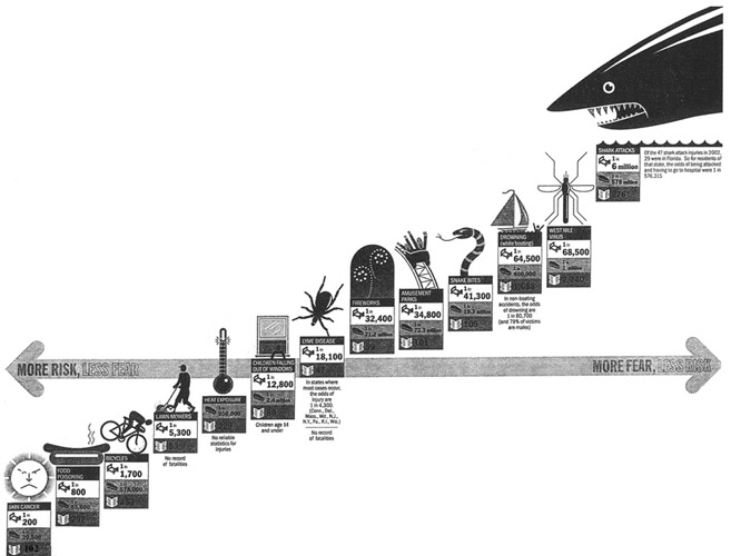
Risk expert David Ropeik and graphic designer Nigel Holmes have combined creative forces to describe the way that our emotional fears can cloud our reasonable perception of risk. "When asked in the abstract about the term 'risk', Americans correctly tend to talk in terms of statistical probability," the article states. "Yet when they are faced with specific threats, emotion overrules logic pretty quickly--we fear the unlikely and are relatively unconcerned about the truly dangerous." To illustrate this the authors provide the following graphic:

For each risk category (e.g., skin cancer, fireworks, west nile virus) there are three pieces of information: risk of injury and of death, and "fear index", as measured by the number of news stories about the topic written last summer. While the companion graphic employs some clever ways to visually present these ideas, it unfortunately has (at least) two logical problems.

First, the graphic presents the information along a line, implying a linear relationship that doesn't exist. While in several cases it is true that high risk activities have a fairly low fear index, and low risk activities have a high fear index, the relationship is by no means linear. The horizontal axis that reads on the left "More risk, less fear" and on the right, "More fear, less risk" only reinforces this misconception.

Second, while the risks decrease from left to right (which agrees with the horizontal axis labels), the risk categories themselves are "plotted" as a line that rises from left to right. Meanwhile except for the extreme "drowning" and "west nile virus" categories, the fear index is comparatively flat and not in any particular order. Finally, with a risk-fear correlation of -0.19, one wonders if the whole thing was worth the bother (except perhaps as an example of the kind of misleading, alarm-causing presentation to avoid!)

Here is the information in the graphic provided by an old-fashioned table.

DISCUSSION QUESTIONS:

( 1) Do you think that the "fear index" as described in this article is a useful measure? What do you think the fear index of terrorism is?

(2) What do you like about the graphic display? How would you improve it?

It's a longshot, but Pepsi might make someone a billionaire Sunday.
The Journal News, 13 September 2003
Abigail Linkgbeil

The Journal News article was written before the Pepsi-Cola Billion Dollar Contest and was the only one we could find that gave a clear explanation of how the contest would be carried out. Our discussion was written after the contest.

On September 14, 2003, the culmination of the Pepsi-Cola Billion Dollar Contest was aired on television in the United States. Here are the rules of the contest. Anyone in the United States could enter the contest in one of several ways. After the entry deadline passed, Pepsi-Cola picked at random 1000 of the approximately 4 million who had entered the contest and flew them to Orlando, Florida). When these 1000 contestants arrived in Orlando, they were each asked to choose a six-digit integer. The company made sure that no two of the chosen integers were equal; if someone chose an already chosen integer, they were asked to choose a different integer. (What is the probability that at least one of the contestants was asked to re-choose?)

After these integers were chosen, a special number, which we'll call the company's number, was chosen on TV. Here's how this was done. Four people stood before the camera. The first held a box of 10-sided dice, the second picked which die to roll (a different die was rolled on each subsequent roll), the third picked up the die and handed it to the second, who rolled it, and the fourth put a billiard ball containing the outcome of the roll into a bag. (Idle question: There are no billiard balls with the number 0 on them. Also, no 0 came up. Did they have special billiard balls with 0's?)

After six billiard balls were in the bag, it was shaken for about 10 seconds (is this enough to randomize them?) Then a chimpanzee was brought into the room, and s/he picked one ball at a time out of the bag. This produced the ordering of the six digits and hence the company's number. (What would they have done if the chimp had picked out two balls at once?) It is claimed the the Chimps were screened for lack of intelligence. Click here to see why this was necessary.

The viewers at home saw the number that was picked, but the contestants did not. Of course, the viewers did not have a list of the 1000 numbers that the contestants had picked, so at this point the only people who knew if one of the contestants' numbers matched the company's number were the people running the show.

The ten who were chosen were those ten whose numbers were 'closest' to the company's number, under the following metric. The first criterion is the number of positions in which the company's number and the contestant's number agree. So, for example, if the company's number were 129382 and the contestant's number were 922384, then there are three positions in which the two numbers agree, namely the second, fourth, and fifth positions. If two numbers are equally close to the company's number using this criterion, then a second criterion was used in an attempt to break the tie.

The digits that matched under the first criterion were removed from both the contestant's and the company's number. In the above example, this would leave the company with the number 192 and the contestant with the number 924. The number of digits in the contestant's new number that matched any digit in the company's new number was recorded. In the present example, there are two such digits, namely 9 and 2. If there was still a tie, say between contestants A and B, then their original six-digit numbers and the company's number were considered as integers, call them a, b, and c, and the quantities |a-c| and |b-c| were calculated. The winner was the contestant with the smaller quantity. It should be clear that at this point it would not be possible to have more than two contestants still tied. If two contestants are still tied, the one with the numerically smaller number was chosen.

The ten finalists were brought up on stage. Each finalist was given a buzzer. There commenced nine rounds. In each round, exactly one finalist was eliminated. The winner was the one who remained after nine rounds. In round number n, the contestants were shown (10000)(n+1) dollars. All contestants who started the round were then given a certain amount of time (either 10 seconds, 20 seconds, or a minute, depending upon the round) to decide whether or not they wanted to take the money and eliminate themselves. During the time period allotted to that round, any contestant could buzz their buzzer, and the first one that did so would claim the money. The other contestants would move on to the next round. If no one buzzed in a given round, the finalist whose number was furthest from the company's number, under the metric described above, was eliminated and won nothing.

Of the ten finalists, three were women and seven were men. All three women buzzed, thereby receiving money. Three of the seven men buzzed, and four (including the eventual winner) never buzzed. All of the women buzzed before any of the men did.

The last finalist remaining was guaranteed one million dollars and had a chance to win one billion dollars. The remaining finalist was given all ten of the finalists' numbers. This last finalist would win one billion dollars if and only if one of these ten six-digit numbers exactly equaled the company's number. The million dollars would be paid in full but a person winning the billion dollar would have the following two options: accept an immediate payment of 250 million dollars or a 40 year annuity with the majority of the money paid out in the 40th year.

When the game was actually played, no one buzzed in the first, second, or ninth round. The winner, a man from West Virginia, had actually chosen the winning number, but it did not equal the company's number, so he won only(!) a million dollars. The winner chose his number, which was 236238, by starting with the bible reference Acts 2:38, which was important to his church. He then changed the letters to numbers by pretending to dial them on a touch-tone telephone. (The company's number was 178238.) Again, for suspense, the numbers were compared one number at a time in reverse order, making the first four numbers the same.

In her Journal News article, Klingbeil reports that Pepsi-Cola will be responsible for the million dollar prize but had purchased an insurance policy from Warren Buffet's Berkshire Hathaway Group who would be responsible for paying a billion dollar prize. She says that our friend Robert Hamman founder of SCA, helped stipulate the game and arrange the deal between Pepsi and the Berkshire Hathaway Group. On the SCA website it is said that the insurance was less than 10 million dollars.

The probability that the billion dollar prize was won was 1/1000. This is because there are a million possible numbers and, if any one of the 1000 participants had chosen the company number, he would have been one of the chosen ten and his winning number would have been available to the million dollar winner. Since the billion dollar prize was really only worth 250 million, the expected loss to Pesi-Cola is 250 thousand. In his talk in our 2000 Chance Lectures, Hamman remarked that the amount for such an insurance policy had less to do with the expected value than what the customer was willing to pay.

DISCUSSION QUESTIONS:

(1) Suppose that the company wanted to make sure that the billion-dollar prize would not be awarded. Can you imagine how they might guarantee this? You may assume dishonesty on the part of any set of people that you wish. Please understand that Chance News is not implying that any dishonest actions occurred.

(2) If you are one of the 1000 contestants, is it true that you have a 1 in 100 chance of being chosen no matter which six-digit number you choose?

(3) Some of the finalists who 'buzzed,' thereby eliminating themselves, did so long before the end of the time period for the round. Does it make sense to buzz early?

(4) What is the probability that someone would win one billion dollars under the rules of the game described above?

(5) Can you calculate the probability that the eventual winner actually picked the number that was closest to the company's number? (You may assume that six of the ten contestants eliminated themselves by buzzing during a round.)

(6) The contestant number that was closest to the company's number matched in four digits. The other two digits in the winning number did not equal the two other digits in the company's number. If 1000 six-digit numbers are picked at random, what is the probability that none of them exactly match the company's number in at least five
locations?

(7) How might one determine whether the fact that all of the women
buzzed before any of the men did is significant?

(8) As we remarked, the SCA reported that the cost of the insurance was "less than 10 million." Does that suggest that it was more than 9 million? What is the expected loss for the Pepsi company considering only the billion dollar prize? Should the cost be based in this? If no, why not?

Video-game killing builds visual skills, researchers report.
The New York Times, May 29, 2003, page A1
Sandra Blakeslee

Action video game modifies visual selective attention.
Nature, Vol. 423, 29 May 2003, pp. 534-537
C. Shawn Green and Daphne Bavelier

Does playing action video-games--especially the first-person shooter variety--improve one's visual attention skills? Researchers Bavelier and Green devised several experiments to study this question and, as reported in the Times article, found that "experienced players of these games are 30 percent to 50 percent better than non-players" on a number of tasks related to visual attention. While they note in their Nature article that "perceptual learning, when it occurs, tends to be specific to the trained task," here the apparently enhanced abilities are in skills that are not uniquely associated with video-game expertise.

Dr. Bevalier, who is an associate professor of cognitive neuroscience at the University of Rochester, led the study. In one experiment, video game players (VGPs) and non-players (NVGPs) were briefly shown between one and 10 squares on a display screen and were asked to report how many had appeared. VGPs significantly out-performed NGVPs (78% vs. 64% accurate, P < 0.003) whenever the number of squares exceeded the NVGPs subitizing range--that is, the number of items that they could immediately perceive (without counting). Furthermore, VGPs could subitize more squares than NVGPs--4.9 vs. 3.3, on average.

Another experiment examined differences between VGPs and NVGPs in sequential processing through what is called "attentional blink". This refers to the difficulty in detecting a second-target object when it appears only a few hundred milliseconds (ms) after a first target. Here subjects were shown a series of black letters in a rapid stream (15 ms for each letter, 85 ms between letters), in which a white letter was randomly positioned (after between seven and 15 letters). Among the eight letters following the white letter, a black "X" appeared 50 percent of the time. Afterwards the subjects were asked to identify the white letter and whether an "X" appeared. The variable of interest was the number of "X"s detected, given that the white letter was correctly identified.

When the "X" appeared up to five letters past the white target, VGPs performed significantly better than NVGPs. For example, according to the box- plot graph that appears with the Nature article, when the "X" appeared two letters past the white letter, VGPs could detect it (after correctly identifying the white letter) about 70% of the time, versus about 35% of the time for NVGPs.

Along with comparing the abilities of VGPs and NVGPs, Bevalier and Green conducted a "training experiment". One group of NVGPs played an action-type game, while a control group played a non-action type, for one hour per day on ten consecutive days. While all participants improved their video-game playing abilities, the players of the action-type game improved their general visual skills significantly more than trainees in the control group.

DISCUSSION QUESTIONS:

(1) The researchers state that, "although video-game playing may seem rather mindless, it is capable of radically altering visual attentional processing." Does this conclusion seem justified? According to the Times article, "among novices, the effects [of the training] waned within a couple of months." How would you answer now?

(2) With respect to the attentional blink experiment, why do you think the researchers had subjects identify the white letter before looking for the "X"? Do you think it matters which white letter is shown? Should all subjects be shown the same letter? Why or why not?

(3.) A footnote on methods in the Nature article says that the number of trials per condition in the attentional blink experiment was eight. If the VGPs were just guessing, what is the chance that they would have achieved 70% (or better) when the "X" appeared two letters past the white letter?

The game show problem vs. the probability problem*
Ask Marilyn, Parade Magazine, July 13, 2003

*After you go to this link choose "Columnists" and then "Marilyn vos Savant."

In an earlier column, (Parade Magazine, 18 May, 2003), an "Ask Marilyn" reader, who lectures in psychology at Erasmus Medical School in the Netherlands, described a variant of the Monty Hall problem that was posed by a student in one of his classes:

Suppose I am taking a multiple-choice test. One question has three choices. I randomly choose A. Then the instructor tells us that C is incorrect. Should I switch to B before turning in my paper?

Marilyn originally gave a brief answer: it doesn't matter if you switch. Apparently her answer surprised and confounded some people--including, Marilyn says, mathematicians-- because of the question's similarity to the Monty Hall problem (in which switching is the favorable option.) There is, however, one significant difference: the instructor doesn't know what choice the student has made before removing one of the three options, while Monty explicitly knows which door a contestant has chosen and never shows what is behind this door.

Specifically, in the Monty Hall problem, 1/3 of the time a contestant will pick a goat at first. Put another way, 2/3 of the time the car is behind one of the other two doors. Once a goat is revealed--but not your pick--the 2/3 chance still holds but can only apply to the other closed door. Thus a contestant wins by switching 2/3 of the time.

Similarly, anyone guessing on the multiple choice test has a 2/3 chance of being wrong. However, 1/2 of the time one's initial (wrong) choice is eliminated, and there's still a 1/2 probability of picking the right answer from the remaining two possibilities. Thus here one can "win" by switching in two ways: by changing to the correct answer when one's first choice is eliminated, which happens 2/3*1/2*1/2 = 1/6 of the time; or by changing to the correct answer when one's first choice isn't eliminated, which happens 2/3*1/2 = 1/3 of the time. In total, you win by switching 1/3 + 1/6 = 1/2 of the time.

Here's Marilyn's explanation:

In the game show problem, the host chooses which door to open based on your choice. Say there's a goat behind doors #1 and #3. If you choose door #1, the host will open door #3. If you choose door #3, the host will open door #1. In the classroom problem, the instructor does not make a statement that an answer is incorrect based on your choice. He isn't even aware of your choice. Instead, he merely announces to the class that one of the answers is incorrect.

DISCUSSION QUESTIONS:

(1) Do you think Marilyn's explanation is correct? Is it convincing?

(2) In the multiple-choice test scenario described, would you switch your
answer? Why or why not?

Who Knew? Time to hit the panic button? How we decide what's risky?
National Geographic, September 2003
Joel Achenbach

Noting that "modern life requires us to be risk analyzers"Achenbach relates a remarkable story about a man who sat calmly reading the a Washington, DC park bench reading the newspaper on the fateful morning of 9/11, even as the Pentagon was on fire and evacuations underway. This unflappable fellow had apparently sized up the situation and concluded that the attack was over!

The article goes on to discuss some of the famous psychological studies that have shown how our intuitive responses to risk often prevail over analytical reasoning. In one experiment, subjects could win a dollar by drawing a red jelly bean from one of two bowls. The first had 100 beans, 7 of which were red; the second had 10 beans, only one of which was red. A majority of subjects preferred the first, even knowing that the odds were worse, because on some emotional level the chances seemed better. Professionals do not necessarily fare better. When asked when to release a patient from a mental hospital, clinicians were more likely to consent when the patient's chance of becoming violent was given as 20% than when that same risk was described by saying 20 patients out of 100 become violent.

The online article contains a pointer to related discussions. One is the University of Delaware's Disaster Research Center, which maintains an extensive set of links to research groups and news outlets that track disasters.

Achenbach's bottom line advice: "Analyze your situation. Crunch the numbers. But don't be so logical you forget to run for your life."

DISCUSSION QUESTION:

(1) If you saw a man sitting quietly on a park bench during a municipal disaster, would you think he had a good internal risk barometer?

The truth about polygraphs.
Boston Globe Magazine, 3 August 2003
Charles P. Pierce

In 2003, the National Academy of Sciences released a report entitled The Polygraph and Lie Detection. As stated in the executive summary, the goal was specifically "to conduct a scientific review of the research on polygraph examinations that pertains to their validity and reliability, in particular for personnel security screening " The report concludes that the use of polygraphs is more problematic in screening job applicants than in questioning criminal suspects, because there is not specific incident under investigation.

In light of this, the Globe Magazine asks why government agencies are still relying on polygraphs in hiring decisions. In 1988, the Employee Polygraph Protection Act banned such use of polygraphs by private businesses. But the article begins with a long anecdote about a candidate who was rejected by both the DEA and FBI, apparently on the basis of shaky polygraph testimony concerning his drug use as an adolescent.

In the wake of the 9/11 terrorist attacks, some people have concluded that we need to take every measure possible to screen government employees entrusted with public safety. According to statistician Stephen Fienberg, who headed the NAS panel "A crisis mentality permeated everything, and it still does. The mystique of this machine always has overpowered the science of it, and now it does especially." Nevertheless, the article points out that the infamous spies Aldrich Ames and Robert Hanssen were able to beat lie detector tests.

This is a long essay, containing many other interesting details about the invention of the lie detector and its historical uses. Here is one more quote, this one from Richard Nixon, who had the following to say about his use of polygraphs to screen staffers: "I know they'll scare the hell out of people."

DISCUSSION QUESTION:

The article quotes John Consigli, a polygraph expert for the Massachusetts State Police, who defends the use of polygraphs as an investigative tool: "We know that a polygraph is between 90 and 98 percent accurate, given a competent examiner and using the latest equipment." What do you understand these percentages to mean?

Antonio Llavelha asked us the following question: If you toss a coin n times, what is the probability that the number of heads that turn up is prime?

This problem was suggested to Antonio by an example in Feller's Introduction to Probability Theory and its Applications 3rd edition p 277, where Feller finds the probability that the number of successes in n Bernoulli trials is an even number.

Peter Doyle's Friday afternoon seminar attempted to answer Antonio's question. Recall that the prime number theorem tells us that the number of prime numbers between 1 and n is asymptotically n/log(n). This says that, if we pick a number at random between 1 and n, the probability that the number is prime is asymptotically 1/log(n). Our first idea was that it should be easy to prove that the probability that the number of heads in n tosses of a coin is prime should also be asymptotically 1/log(n).

If we toss a coin 2n times, the expected number of heads is n and the standard deviation is 1/(sqr(2) sqrt(n)). Thus the central limit theorem tells us that most of the distribution is concentrated on intervals of the form [n - c sqr(n), n+c sqrt(n)] where c = 3/sqr(2). The prime number theorem suggests that the number of primes in this interval should be asymptotically (2c sqr(n))/log(n). Thus the ratio of the number of primes in this interval and 2c sqr(n)/log(n) should approach 1 as n tends to infinity. Here is alog plot of this ratio for n = 10³ to 10¹³:

So it looks hopeful. We decided that to prove that this ratio does converge to 1 it would be sufficient to prove that the number of primes in the intervals [n, n +sqr(n)] is asymptotically sqr(n)/log(sqr(n).

Then one Friday the department's new number theorist, Carl Pomerance, wandered into our seminar assuming, from the laughing he heard, that it was a party. Peter asked him what he knew about the asymptotic behavior of the number of primes in the interval [n, n +sqr(n)]. Carl's first remark was: "we don't even know if there are any primes in these intervals." Then he explained why we don't. For p a prime, let g(p) be the number of composite numbers between p and the next prime number. In a sequence of papers it has been shown that g(p) does not grow faster than p^f+e) (for every e >0) for successively smaller values of f. The smallest value known to-date is f = .525. So we have to wait for better results to say that all intervals [n, n+ sqr(n)] have prime numbers. When these gap theorems are proven, it is often also shown that the number of primes in intervals of the [n , n+n^f] is asymptotically n^f/log(n). The best result for this so far is f = 7/12 =.5833. If they ever get f down to 1/2 here, we be able to prove the conjecture that if we toss a coin n times the probability that the number of heads is prime is asymptotically 1/log(n).

Since we have failed to answer Antonio's question let's at least show how to obtain Feller's result for the probability of getting an even number when you toss a biased coin with probability p for heads n times. For p = 1/2 the answer is 1/2. To see this write down all sequences of H's and T's of length n that have an even number of successes. Now change the first element of each sequence and you will get all sequences with an odd number of successes. Thus 1/2 of the possible sequences have an even number of heads, and so the probability that in n times of a coin the number of heads is even is 1/2.

For the general p let q = 1- p and let p(n) be the probability that in n tosses we obtain an even number of heads. Then Feller proved:

p(n) = 1/2 + 1/2(q-p)ⁿ

He used the following recursion equation for n >= 1,

p(n) =q p(n-1)+p(1-p(n-1)) = p + (q-p)p(n-1)

with p(o)=1.

Of course we can just check that Feller's solution satisfies this equation but it is more interesting to derive his solution. There are several different ways to do this. Feller uses generating function. We could also treat this as a two-state Markov chain. However, it seems simplest to us to note that we have a linear difference equation, so the solution is the sum of the solution to the homogeneous equation h(n) = (q-p)h(n-1) and a particular solution for the equation for p(n). The solution to the homogeneous equation is h(n) = h(0)(q-p)ⁿ. It is easy to check that p(n) = 1/2 is a particular solution to our original difference equation. Thus the general solution is p(n) = 1/2 + h(0)(q-p)ⁿ. Using the fact that p(1) = q we see that h(o) = 1/2 giving Feller's solution p(n) = 1/2 + 1/2(q-p)ⁿ.

In Chance News 12.03 we discussed a coincidence problem of Brian Hayes for which Brian had to compute the probability of three or more people having the same birthday when there are n possible birthdays. We remarked that this is a more difficult calculation that for a match of two or more birthdays. Roger Pinkham wrote us:

It got me thinking about something that has long fascinated me, the birthday problem. It has always surprised me that no one (excepting me) to my knowledge has observed the following.When dealing with the classical case there are r(r-1)/2 pairs if you have r people. The probability the pair have coincident birthdays is 1/365. If you regard this as a Poisson with mean m = r(r-1)/(2*365), then exp(-m)=0.5 exactly matches the usual approximation. More importantly it opens the way for the 3 coincident birthdays case. Given n cells and r balls, the mean number per cell is m = r/n and[(1+m+m^2/2)*exp(-m)]^n provides 0.490175 for n=365 and r=88, while the exact answer is 0.488935. r=87 pops you over the top for each. Not bad for an easy approximation.

We wanted to see how the method Roger used for 3 matches would work for larger number k of matches and compare it to other such computations. Let's call the smallest number that gives a probability greater than or equal to 1/2 for at least k matches the kth "critical number." The methods that have been used to compute the critical values are discussed in an article by S. Finch, based on work of Patrice Le Conte, available here.

Finch presented an algorithm for computing the critical values and remarked that this took exponential time in k. Peter Kostelec implemented this algorithm and found that it was not practical to use this for values of k greater than about 10. Finch provided exact values up to k = 15 saying that they were computed by Bruce Levin using a method using results he had proven about multinomial distributions. Levin described his method in his paper "A Representation for Multinomial Cumulative Distribution Functions",The Annals of Statistics, Vol. 9, No. 5, 1123-1126. When we looked at Levin's method we found that it was similar to Roger's but provided exact values.

We found Levin's method very elegant so decided to describe it here. We need to remind you what a multinomial distribution is. Since math is hard to show using html, we have borrowed the definition of a multinomial distribution from here.

The values p₁,.., p_k are called the "parameters" for the distribution. Familiar examples of such distributions are obtained from tossing a coin n times and counting the number of heads and tails that occur, or rolling a die n times and counting the number of times each of the numbers from 1 to 6 turns up. If we number the possible birthdays from 1 to 365, then we can consider a person's birthday as the result of rolling a 365-sided die. So in a group of n people, the number of times that each possible birthday occurs has a multinomial distributions with parameters p_i = 1/365 for i = 1 to 365. Then X_i is number of people with the ith birthday. It has a binomial distribution with probability of success = 1/365 and expected value n/365. Note that the sum of the X_i is 365, so these are not independent random variables.

To solve the birthday problem for k matches, we want to find the smallest number N of people we have to have to have a probability greater than 1/2 of having k or more people with the same birthday. We do this by finding the probability that we do not have k or more matches. Thus we want to find the smallest k such that

(1)   P(X₁ <= k-1, X₂<= k-1,....,X365<= k-1) < 1/2

For his approximation, Pinkham approximated the binomial distribution by a Poisson distribution with the same mean and assumed that they were independent. Levin avoids these approximations by using the fact that any multinomial distribution can be obtained by replacing the random variables X_i by random variables Y_i with a Poisson distribution having the same mean and then conditioning on the sum of the Y_i = N. Levin then obtains a formula for the probabilities (1) from which we can compute the critical values. To obtain this formula he uses only Bayes theorem P(A|B) = P(A)/P(B)P(B|A). It is such a simple argument that we decided to include it here.

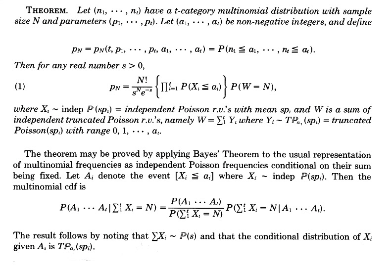
Note that the Poisson random variables do not have to have the mean of X_i but it is natural to take s = N so that they do. The first two terms in his formula for p_N are easy to compute. The third term requires finding the probability that the sum of N independent random variables with a truncated Poisson distribution is equal to N. A truncated Poisson distribution is a Poisson distribution given that the outcome is less than or equal to a prescribed number. Levin remarks that, for small values of k, the convolution can be computed and for larger values the central limit theorem can be used to obtain an approximate value.

Note that Pinkham's approximation amounts to using only the center term in Levin's formula.

Charles Grinstead implemented Levin's method in a way that made the computation time to calculate the convolution polynomial in k and so using his program we can calculate exact values for reasonably large n. Doing this we compared Pinkham's approximation and the exact values for values of k from 2 to 25. We note that his approximation is quite good.

Study says 1 in 7 women in state has been raped.
Manchester Union Leader, 21 August, 2003
Kate McCann

Another view: One in seven NH women raped? I don't think so.
Manchester Union Leader 26 August, 200, guest commentary
Michael R. Bowen: medical doctor in Wolfeboro.

Rape in New Hampshire: A report to the state. One in seven.
Prepared by National violence against women prevention research, 15 may 2002
Dean G. Kilpatrick, Kenneth J. Ruggiero

The first Union Leader article reports the following information about the study carried out by Dean Kilpatrick and Kenneth Ruggiero:

One in seven women in New Hampshire has been forcibly raped, according to a study by the National Violence Against Women Prevention Research Center. Victim advocate groups say that figure includes women older than 18 and doesn't take into account minors. The study used national data from two separate studies, one conducted in the 1980s and the other in the 1990s that found common factors among women who said they were raped. Those numbers were applied to current census data. One in seven women translates to 65,000 women in the state, the center's report said, saying New Hampshire's statistic is slightly higher than the national average.

On the basis of this sketchy information about the study, Dr. Bowen provides the reader with the third sentence above "The study used national data..." and then describes the study's methodology as:

They found two old studies which identified "common factors" among women who said they were raped. Then they went to the census, found the number of women with those characteristics and declared them raped.

Bowen goes on to say:

The underlying premise of the study is a whopping fallacy: that if you identify some common characteristics among people who have a certain thing happen to them, then anyone who has those characteristics will have that thing happen also.

He then gives the example:

Look at it this way: almost all of our combat casualties of the last 60 years have been male, ages 18-30, wearing green clothes, and carrying a weapon. We can apply the logic of this "study" to determine that most of our servicemen in Iraq have been shot.

So we have the original Union Leader article in which the readers get only a vague idea of how the study was done and then another article by a guest commentator who gives a ridiculous interpretation of what the original article said, but in a way that will seem believable to many of the readers.

So, of course, we were curious as to how the study was done. The Kilpatrick- Ruggiero report to the state provides this information. Their report was indeed based on combining the results of two national studies: the National Women's Study (NWS) and the National Violence Against Women Survey (NVAWS). The NVAWS study was sponsored by the National Institute of Justice (NIJ) and the Centers for Disease Control and Prevention (CDC). These surveys were given to adult women (age 18 older). In their report Killpatrick and Ruggiero write:

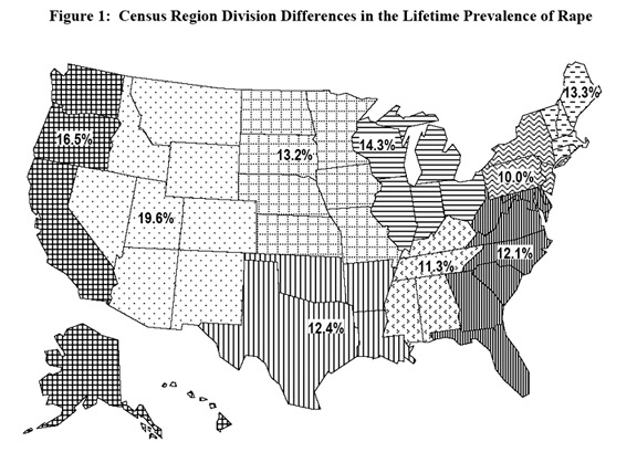
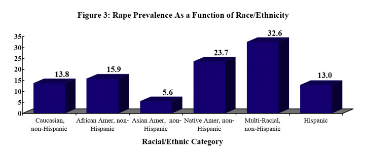
Data from these studies indicate that approximately 13.4% of adult women in the United States have been victims of completed forcible rate sometime during their lifetime. These studies also found that risk of having ever been raped was related to a women's current age, her race/ethnicity, and the region of the nation she currently lives in. Both studies also found that the majority of rapes these adult women had experienced occurred when they were under the age of 18.

They present the following graphics to illustrate these risk factors.

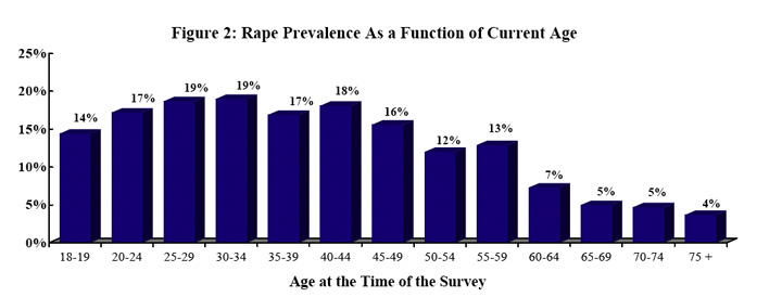
The fact that the increase with increasing age is modest can be accounted for by the fact that over half of the rapes took place when the women was less than 18 years old. However, the decrease in older women is more mysterious. We would assume that women who had lived longer would have had a higher chance of having been raped. Various explanations have been offered for this such as, the incidence of rape is greater now then when these older people were young, or older people are more reluctant to admit having been raped.

Using the data for all the census regions, the authors used logistic regression to obtain estimates for the probability of rape during lifetime for an adult women in a specific census region, in a specific age range, and of a particular race/ethnicity. Then they used the 2000 census to estimate for New Hampshire the number of people in the various age ranges and race/ethnicity categories. From this and the results of the regression, they obtained the estimate that adult women in New Hampshire have a 13.7% chance of being raped sometime during their lifetime. Hence the one in seven estimate.

There have been a number of other estimates of the incidence of rape and while they all are are depressingly high there has been considerable interest in why the estimates are so different. For a detailed discussion of this problem see "Researching the "Rape Culture" of America by Christina Hoff Sommers.

Since 1972 the Bureau of Justice Statistics (BJS) has carried out an annual survey called the National Crime Victimization Survey (NCVS). This survey measures property crimes and the violent crimes of rape and sexual assault, robbery, aggravated assault, and simple assault. Two times a year, U.S. Census Bureau personnel interview household members in a nationally representative sample of approximately 42,000 households (about 76,000 people). Approximately 160,000 interviews of persons age 12 or older are conducted annually.

Ronet Bachman (1) compared the results relating to the annual incidence of rape from the 1995 NCVS survey and the NVAWS survey. She reports that the estimate for the total number of rapes experienced by adult women for the NVAWS survey was 876,064 (95% confidence interval (443,772, 1,308,356) compared with 268,640 (95% confidence interval 193,110 to 344,170) for the NCVS. Since the confidence intervals do not overlap she considered these differences significant. Bachman gives a number of reasons that might account for this difference. She suggests that the context of the surveys might make a difference. The NVAS was presented as a survey interested in a number of personal-safety-related issues while the NCVS, as the name conveys to respondents, is a survey interesting in obtaining information about crimes. She remarks that "Unfortunately, some survey participants still may not view assaults by intimates and other family members as criminal acts. Bachman also discusses differences in the screening questions that could make a difference. In particular the NVAWS survey has four difference descriptions of a rape as compared to one for the NCVS.

We asked Michael Rand, Chief of Victimization Statistics, Bureau of Justice Statistics, to comment on these differences and he wrote:

As far as NCVS/NVAWS comparisons of rape estimates, when confidence intervals are constructed around the estimates from the two surveys, there is not much difference between them. There are a number of methodological reasons why the estimates do differ to the degree that they do. One thing to remember is that the annual incidence estimate from the NVAWS is based upon a very small number of cases. (I believe it is 27, but could be off by a few.) Also, it was an estimate for 1995 (approximately; interviews were conducted in late 95 and early 96 and they referred to the previous 12 months.) So the data are old and should not be used as an annual estimate for all time, because crime rates have changed tremendously since then.

In the report "Criminal Victimization, 2002," the authors include the following graph to show from the NCVS surveys the changes over all victimizations from 1973 to 2002:

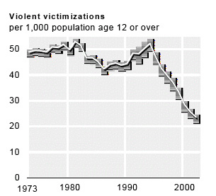
The report reports that the rate for rape was 1 per 1,000 persons age 12 or older in 1993 and .4 peer 1000 persons in 2002. Of course the New Hampshire report dealt primarily with the incidence of rape in the lifetime of women and it is not clear how much the decrease in annual rate might effect their conclusions. However, the authors of the New Hampshire report do stress that what is really needed is an up-to-date survey.

REFERENCES

(1) Ronet Bachman. 2000. A comparison of annual incidence rates and contextual characteristics of intimate-partner violence against women from the National Crime Victimization Survey (NCVS) and the National Violence Against Women Survey (NVAWS). Violence Against Women, 6(8), 839-867.

DISCUSSION QUESTIONS:

(1) Do you think the differences in the rape rate between census regions are significant? How could you get check this?

(2) The NCVS found that marital status is also an important risk factor for rape. In particular women who are separated from their husband have a higher rate of rape. Can you think of other risk factors that might have been included in the New Hampshire report? Do you think it is important to have more risk factors in making such a report? Why?

The GNU probability book.

This introductory probability book, published by the American Mathematical Society has, since publication, also been freely available on from our book website We are pleased that this has made our book more widely available. Other resources for using this book in class such as solutions to problems, errata and computer problems can also be found on the book website.

Thanks to the efforts of our colleague Peter Doyle, we are pleased to announce that our book has now been made freely redistributable under the terms of the GNU General Public License (‘GPL’), as published by the Free Software Foundation: Peter has written some remarks on what copyleft means as an appendix to the GNU version of our book. Here Peter writes:

The GPL is the original ‘copyleft’ license. Briefly stated, the GPL permits you to do whatever you like with a work, as long as you don’t prevent anyone else from doing what they like with it.

Thanks

We owe our ability to distribute this work under the GPL to the far-sightedness of the American Mathematical Society. We are particularly grateful for the help and support of John Ewing, AMS Executive Director and Publisher.

At another level, we owe our ability to distribute this work under the GPL to Richard Stallman: inventor of ‘copyleft’; creator of the GPL; founder of the Free Software Foundation. Copyleft is an ingenious idea. Through the GNU/Linux operating system, and scads of other computer programs, Stallman’s idea has already had a profound impact in the area of computer software. We believe that this idea could transform the creation and distribution of works of other kinds, including textbooks like this one. The distribution of this book under the GPL can be viewed as an experiment to see just where the idea of copyleft may take us.

Click here for the complete version of Peter's explanation of copyleft and the GNU License.

The AMS continues to distribute a version of this book in printed form: Those who wish to have the published version of our book are invited to contact the AMS bookstore. For those using the book in class we will keep on our book website a pdf version essentially identical to the published version.

Of course we hope that the GNU version will become better than the present published version. The current GNU version is, available here, in pdf format. A bundle of source files can be found here and an index for the material related to the GNU book can be found here.

We hope that having our book under the GNU contract will enrich our book and encourage others to make use of material from our book in their own writing. We will keep a list of contributions to the GNU version of the book website and will welcome additional contributions.

Here are the first contributions to the GNU version of our book.

Kemeny's Constant: Peter Doyle.

This discussion relates to Exercise 24 in Chapter 11 concerning "Kemeny's Constant" and the question: Should Peter have been given the prize?

Hedging Huygens: Peter Doyle.

In the historical remarks for section 6.1, Grinstead and Snell describe Huygen's approach to expected value. The were based on Huygen's book The Value of all Chances in Games of Fortune which can also be found here. Peter reworks Hygen's discussion to show connections with modern ideas such fair markets and hedging. He illustrate the limitation of hedging using a variant of the St. Petersburg Paradox.

A local limit theorem for sampling without replacement: Marvin Pinsky

In Feller's Introduction to Probability theory and Its Applications, volume 1, 3d ed, p. 194, exercise 10, there is formulated a version of the local limit theorem which is applicable to the hypergeometric distribution, which governs sampling without replacement. In the simpler case of sampling with replacement, the classical DeMoivre-Laplace theorem is applicable. Feller's conditions seem too stringent for applications and are difficult t to prove. It is the purpose of this note to re-formulate and prove a suitable limit theorem with broad applicability to sampling from a finite population which is suitably large in comparison to the sample size.

Other resources related to our book including answers, errata and computer programs can be found on the Grinstead-Snell book website.

Copyright (c) 2003 Laurie Snell

This work is freely redistributable under the terms of the GNU General Public License published by the Free Software Foundation. This work comes with ABSOLUTELY NO WARRANTY.