Statistical Ideas

• Linear Regression
• Multiple Regression
• Histograms
• Data/Sample Bias

This topic provides a good introduction to analysis of linear and multiple regression on a computer statistical package. The data from different years also may be used in comparative histograms for analysis. JMP was the software used in this write-up. The data and contrasting study results mentioned in part I raises interesting questions about the source of data and bias of the researchers.

Linear Regression

-How to Qualitatively and Quantitatively Look at Two Factors and Determine the Validity of a Linear Model

For this example, use the math SAT scores and numeric grade in Math 3-92 as the and in the scatter plot (Separate data files accompany this profile). In order to set up a scatter plot and perform a regression, select Fit by . Next, select Fit Line to fit a simple regression line through the data points. The regression line minimizes the sum of squared distances from each sample point to the line of fit. It would be useful to next find the value of r, the correlation coefficient, which helps determine if there is a linear relationship between the two variables. To find in JMP, fit any Density Ellipse and check under the Bivariate Statistics (Figure 1).

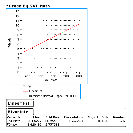
Figure 1: Linear Model

Next, save the Predicteds, the points along the best fit line. Then you can see how far the actual values deviate from the predicted values.

It is also good to save the Residuals which are points measuring the distance of a point from its predicted value. This value is measured vertically. Then plot the residuals under Distribution of Y's and see how they fall under the histogram or normal curve (Figure 2). The closer they come to a bell shape, the better the model. You can also plot the residuals by the actuals under Fit X by Y and see if there is clumping in the upper left and lower right corners (Figure 3) If there is, then there is something wrong with the model because the points should be rather evenly distributed.

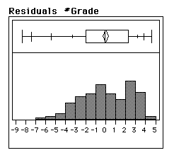
Figure 2: Math 3 Grade Residuals

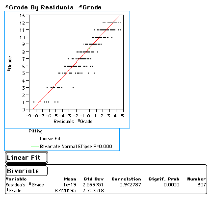
Figure 3: Actual Grades versus Grade Residuals

This two variable method is good for preliminary analysis and should be used to look at the correlation between sex and scores and other combinations. However, for a more thorough analysis, there is multiple regression.

Multiple Regression

-How to Perform Multiple Regression

Select Fit by s to start an analysis of the effects of more than one independent variable. For this example, use the ETS Validity Data and choose SAT Verbal, SAT Math, and Sex as the s (independent variables). (dependent variable) will be Freshman GPA (a.k.a. 1st Yr GPA).

-What the Multiple Regression Summaries Mean

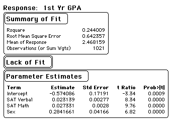
Figure 4: Results of Multiple Variable Analysis

The Summary of Fit (Figure 4) contains some important information. The R square is akin to the r used in the two variable linear correlation. The R square statistic represents the proportion of total variation in freshman year GPA as explained by the regression of freshman year GPA on the independent variables (Pindyck, 61). The smaller R square is, the less your s are accountable for the outcome of . An R Square of 1 would suggest that you have adjusted all the influencing factors and you have a well fit model. A R square greater than 1 does not imply a good fit. The Root Mean Square error is the unit error on each side of the mean for . The Mean of Response is just the mean of . Observations is just the same as the number of rows.

Some other important information is contained under the header, Parameter Estimates (Figure 4). The numbers in the first column after the s are used to create the equation/model we are looking at. For example, freshman year GPA = . One can interpret .023SATV as: controlling for the other variables, a 1 point increase in the SAT verbal score, freshman GPA should be .023 higher. (Note that the intercept is negative when in theory it should be greater than zero- hence our model is far from being comprehensive). Since the number before Sex is positive, this implies that being female has a positive effect on GPA. So, where men and women have the same SAT scores, women can be expected to do better as a freshman in this regression. If sex was irrelevant in this equation the sex coefficient would be zero.

You might also want to save the Predicted Formula, which for JMP is located under the $ icon, because it will provide the formula just described under the estimate column.

Histograms

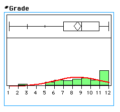
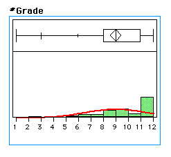
Histograms can be created by selecting the header, Distribution of s, and then assigning a variable. Seeing how the s fall under the normal curve can be useful in comparative analysis. For example, the grades for Economics 1 are provided for classes from 1991 and 1992. It would be helpful to assign the grades as the variable under the curve and compare the curves for both years (Figures 5 and 6). This way it can be observed whether or not there was a significant change in how the grades were distributed from year to year. Doing this for different variables, enables the analyzer to look for other trends while holding constant as many other factors as possible.

Figure 5: Grade distribution for Econ1-91

Figure 6: Grade distribution for Econ1-92

Data/Sample Bias

The ETS has suggested that a purely random sample is next to impossible to acquire for research on the issue of sex bias and the SAT. Examining the samples used in each study outlined in this profile can help determine the validity of the research results.

SOURCES (* indicates possible classroom material)

Baron, Jonathan, and M. Frank Norman. ``SATs, Achievement Tests, And High- School Class Rank As Predictors Of College Performance." Educational and Psychological Measurement, 1992, 52: 1047-1055.

Brush, Stephen G. ``Women in Science and Engineering." American Scientist. September-October 1991, Vol. 79: 404-419.

*Burton, Nancy W., Charles Lewis, and Nancy Robertson. College Board Report No. 88-9: Sex Differences in SAT Scores. New York: College Entrance Examination Board, 1988.

Chatterjee, Samprit, and Bertram Price. Regression Analysis By Example. 2nd ed. New York: John Wiley & Sons, 1991.

Kaufman, Susan. ``SAT-isfaction Not Guaranteed." Chicago Tribune, 12 April 1987: 2C.

Lewis, Charles. Educational Testing Service. Princeton, New Jersey. 1992-93.

Lubetkin, Julie. The Scholastic Aptitude Test: A Valid and Unbiased Predictor of College Performance?, Senior Thesis, Woodrow Wilson School of Public and International Affairs, Princeton University, 1988.

* Piccoli, Sean. ``Charges Persist SATs Biased Against Women and Minorities." The Washington Times, 5 August 1991: G6.

*Rosser, Phyllis. The SAT Gender Gap. Washington DC: Center for Women Policy Studies, 1989: 29-67.

Rowe, Jonathan. ``Scholastic Aptitude Test Scores: Are They Unfair to Women?" The Christian Science Monitor, 20 April 1987: 23.

*Sall, John, Katherine Ng, and Michael Hecht. JMP [computer statistics software]. SAS Institute: Cary [NC], 1989.

*Wainer, Howard and Linda S. Steinberg. ``Sex differences in Performance on the Mathematics Section of the Scholastic Aptitude Test: A Bidirectional Validity Study." Harvard Educational Review, Vol. 62 No. 3 Fall 1992.

Walker, Judge John M. United States District Court for the Southern District of New York. Khadijah Sharif v. New York State Education Department. No. 88 Civ. 8435 (JMW). Lexis 961, Decided 3 Feb. 1989.