This is the third and final issue of our series meant to assist in listening to Peter Sarnak's lecture on the Riemann Hypothesis available at the MSRI website. Parts I and II related to the first part of Sarnak's talk in which Sarnak discusses the history of the Riemann Hypothesis. In the second part of his talk, Sarnak discussed the remarkable connections between the zeros of the zeta function, energy levels in quantum theory, and the eigenvalues of random matrices. Here we will provide some background information for understanding these connections. This part was written jointly by Dan Rockmore and Laurie Snell with a lot of help with programming from Peter Kostelec and Charles Grinstead.
It all begins with a chance meeting at Princeton's Institute for Advanced Study between number theorist Hugh Montgomery, a visitor from the University of Michigan to the Institute's School of Mathematics, and Freeman Dyson, a member of the Institute's Faculty of the School of Natural Sciences, the same department which claimed Albert Einstein as one of its first members. Dyson is perhaps best known as the mathematical physicist who turned Feynman diagrams, the intuitive and highly personal computational machinery of Richard Feynman, into rigorous mathematics, thereby laying the mathematical foundations for a working theory of quantum electrodynamics.
Montgomery had been working for some time on various aspects of the Riemann Hypothesis. In particular he had been investigating the pair correlation of the zeros which we now describe.
Recall that the Prime Number Theorem states that, if ![]() is the number of primes not exceeding
is the number of primes not exceeding ![]() , then
, then
| (1) |
| (2) |
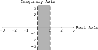
Recall that the non-trivial zeros of the zeta function all lie in the critical strip of the complex plane:
Let ![]() be the number of zeros in the upper half of the critical strip with imaginary part at most T. Of course, if the Riemann Hypothesis (RH) is true then the zeros in the critical strip all lie on the line
be the number of zeros in the upper half of the critical strip with imaginary part at most T. Of course, if the Riemann Hypothesis (RH) is true then the zeros in the critical strip all lie on the line
![]() Then the analog of the prime number theorem for N(T) is
Then the analog of the prime number theorem for N(T) is
| (3) |
We now assume the RH and denote by
![]() the imaginary parts of the first n zeros in the critical region. Then it follows from (3) that
the imaginary parts of the first n zeros in the critical region. Then it follows from (3) that
| (4) |
Montgomery studied the consecutive spacings
![]() between the zeros. He effectively spread them out to obtain normalized spacings
between the zeros. He effectively spread them out to obtain normalized spacings ![]() with mean spacing asymptotically 1. There are two ways that we can do this. We can normalize the zeros in such a way that the gaps will have their mean asymptotically 1 or we can normalize the gaps directly. Following Montgomery [3], Katz and Sarnak [5] use the first method normalizing the zeros by:
with mean spacing asymptotically 1. There are two ways that we can do this. We can normalize the zeros in such a way that the gaps will have their mean asymptotically 1 or we can normalize the gaps directly. Following Montgomery [3], Katz and Sarnak [5] use the first method normalizing the zeros by:
Odlyzko uses the second method. He starts with the unnormalized consecutive spacings ![]() and normalized these by
and normalized these by
This normalization is arrived at by considering more accurate asymptotic expressions for
Montgomery proved a series of results about zeros of the zeta function which led him to the following conjecture.
Let ![]() and
and ![]() be two positive numbers with
be two positive numbers with
![]() . Montgomery conjectured that
. Montgomery conjectured that

The right side
![]() is called a kth-consecutive spacing.
Thus, for the normalized spacings, we are counting the number of kth-consecutive spacings that lie in the interval
is called a kth-consecutive spacing.
Thus, for the normalized spacings, we are counting the number of kth-consecutive spacings that lie in the interval
![]() . Of course this
number can be bigger than 1.
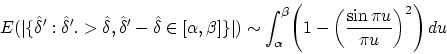
The function
. Of course this
number can be bigger than 1.
The function
If the zeros were to occur at random points on the critical line, i.e. where one zero occurs
has no bearing on where another would occur, then the zeros would act like a Poisson process. In this case the pair correlation function would be the constant function ![]() . On the other hand, Montgomery's conjecture implies that, if we are sitting at a zero on the critical line, it is unlikely that we will find another zero close by.
An analogy is with the prime
numbers themselves - that two is prime implies that it is
impossible that any two numbers separated by one (other than two and three) can both be prime.
. On the other hand, Montgomery's conjecture implies that, if we are sitting at a zero on the critical line, it is unlikely that we will find another zero close by.
An analogy is with the prime
numbers themselves - that two is prime implies that it is
impossible that any two numbers separated by one (other than two and three) can both be prime.
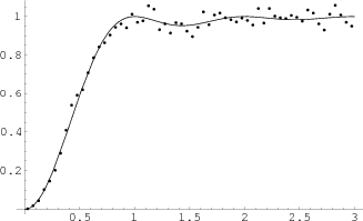
Of course, it is natural to ask if the data supports Montgomery's conjecture. Thanks to the remarkable computations of Andrew Odlyzko we have a large amount of data. Since Montgomery's conjecture is an asymptotic results Odlyzko concentrated on computing the zeros near a very large zero. He has some of this data available on his web site. For example he has the zeros number ![]() through
through
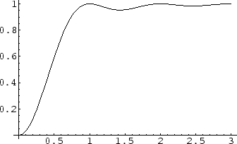
![]() of the zeta function. In Figure 3 we show the empirical results from the data compared with the theoretical limiting density.
of the zeta function. In Figure 3 we show the empirical results from the data compared with the theoretical limiting density.
We have divided the interval from 0 to 3.05 into 61 equal subintervals and used these for our intervals
![]() . We see that the fit is very good for intervals between
. We see that the fit is very good for intervals between ![]() and
and ![]() , but it is less convincing for the other intervals.
, but it is less convincing for the other intervals.
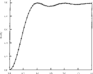
In computations in the 1980's Odlyzko computed 175,587,726 zeros near zero ![]() . More specifically he started with zero
. More specifically he started with zero
![]() and ended with zero number
and ended with zero number
![]() . Using this data, Odlyzko used 70 million zeros near zero
. Using this data, Odlyzko used 70 million zeros near zero ![]() to check Montgomery's conjecture obtaining a remarkable fit as shown in Figure 4.
to check Montgomery's conjecture obtaining a remarkable fit as shown in Figure 4.
Montgomery's work was very exciting, since proving any sort of structure about the zeros - if they are where we think they are - is exciting. But things like this can provide subtle clues towards a proof. Perhaps it is possible to find a way of producing numbers that have the same properties, and if so then maybe, just maybe, you can find some direct link between Riemann's zeta function and the process, and then maybe, really - just maybe you can prove the Riemann Hypothesis. So, did this pair correlation arise in other places?
Freeman Dyson had been working on a problem in statistical
mechanics - this is the physics and mathematics which attempt
to model the behavior of huge systems, like all the atoms in a
liter of gas - all
![]() of them. For systems of
such huge populations it is impossible to model each
particle individually and what statistical mechanics tries to
do is to find some predictable average behavior, or to work
out the rough distribution of what the particles are doing,
say 20% are moving at such and such a speed, in such and such
a direction, so much percent of the time.
of them. For systems of
such huge populations it is impossible to model each
particle individually and what statistical mechanics tries to
do is to find some predictable average behavior, or to work
out the rough distribution of what the particles are doing,
say 20% are moving at such and such a speed, in such and such
a direction, so much percent of the time.
Dyson, along with his collaborator Mehta, had been working out the theory of random matrices. Building on work of another Princetonian (and Nobel laureate) Eugene Wigner, they were looking to gain some insight (and prove some theorems) about the statistical properties of the eigenvalues of a random matrix, which would then cast some light on the problem of the prediction and distribution of energy levels in the nuclei of heavy atoms.
The connection between eigenvalues and nuclei is a bit beyond this discussion; but suffice it to say that the classical many-body formulation of the subatomic dynamics (electrons spinning around a positively charged nucleus) fails. This led Heisenberg to develop a quantization of this classical setting in which a deterministic Hamiltonian, a scalar function describing the energy of a system in terms of the positions and momenta of all the acting agents, is replaced by a matrix acting on a ``wave function'' which encapsulates our uncertain or probabilistic knowledge of the state of our energetic system. It is interesting to note that Heisenberg did not even know what matrices were when he developed his theory. He was completely led to their constructions by physical theories.
In this matrix mechanics, setting the spectral lines which are observed when a nucleus is bombarded with a particular kind of radiation (which corresponds to an effect of resonant radiation) may in fact be predicted as eigenvalues of certain matrices which model the physics. For heavy nuclei the models are too difficult to construct (too many interactions to write down), so the hope is that the behavior of this model might be like that of an average model of the same basic type (symmetry). These average or ensemble behaviors could be calculated and give some insight into the particular situation, or so it was hoped. These were the things that Dyson and Mehta were studying.
In a brief conversation in the Institute tea room, where the ghosts of Einstein, Godel, Von Neumann and Oppenheimer still held forth (although did not eat many of the cookies) Dyson and Montgomery discovered that it looked as though they had been studying the same thing!
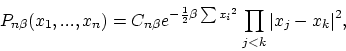
To understand why Dyson recognized the pair correlation function, we need to understand some results about random matrices. A random matrix is a matrix whose entries are random variables. In the areas of quantum mechanics and number theory, there are several classes of random matrices that are of interest; they are referred to by certain acronyms, such as GUE, CUE, GOE, and GSE. In Sarnak's lectures, he discusses the CUE class which is asymptotically the same as the GUE class. Here, we will discuss the GUE class because that is the one chosen by Odlyzko but it turns out that the mathematics is the same.
The acronym GUE stands for Gaussian Unitary Ensemble. By ensemble we mean a collection of matrices and a method for choosing one of them at random. The entries in an ![]() GUE matrix are complex numbers chosen so that the matrix is Hermitian, i.e. so that if the
GUE matrix are complex numbers chosen so that the matrix is Hermitian, i.e. so that if the ![]() th entry is
th entry is ![]() then the
then the ![]() th entry is
th entry is ![]() . For diagonal entries this means that
. For diagonal entries this means that ![]() so the diagonal entries must be real. Thus to pick a random
so the diagonal entries must be real. Thus to pick a random ![]() GUE matrix, we only have to specify how we pick the entries on or above the main diagonal. For a GUE ensemble, we choose entries
GUE matrix, we only have to specify how we pick the entries on or above the main diagonal. For a GUE ensemble, we choose entries ![]() on the main diagonal from a normal distribution with mean 0 and standard deviation
on the main diagonal from a normal distribution with mean 0 and standard deviation ![]() . For entries
. For entries
![]() with
with ![]() (above the main diagonal)
(above the main diagonal) ![]() and
and ![]() are chosen from a normal distribution with mean 0 and standard deviation 1. Then the entries below the diagonal are determined by the condition that the matrix be Hermitian.
are chosen from a normal distribution with mean 0 and standard deviation 1. Then the entries below the diagonal are determined by the condition that the matrix be Hermitian.
It should be noted that some authors choose the entries ![]() on the main diagonal to be a standard normal distribution and the entries above the main diagonal
on the main diagonal to be a standard normal distribution and the entries above the main diagonal ![]() and
and ![]() to have a normal distribution with mean
to have a normal distribution with mean ![]() and standard deviation
and standard deviation ![]() . This choice does not make an essential difference in the results that we will discuss but makes annoying differences in normalization factors.
. This choice does not make an essential difference in the results that we will discuss but makes annoying differences in normalization factors.
It is well-known from linear algebra that Hermitian matrices have real eigenvalues The eigenvalues of a matrix ![]() are numbers
are numbers ![]() such that for each such
such that for each such ![]() , there exists a non-zero vector
, there exists a non-zero vector ![]() with the property that
with the property that
![]() .The first question one might consider is how these eigenvalues are distributed along the real line. More precisely, if we choose a random
.The first question one might consider is how these eigenvalues are distributed along the real line. More precisely, if we choose a random ![]() GUE matrix, can we say anything about the probability of finding an eigenvalue of this matrix in the interval
GUE matrix, can we say anything about the probability of finding an eigenvalue of this matrix in the interval ![]() ?
?
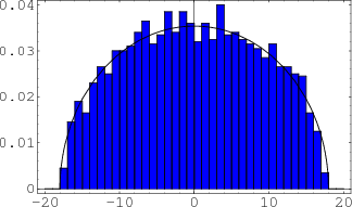
The physicist Eugene Wigner worked with random matrices in connection with problems in quantum mechanics. He proved that as
![]() , the density function of the positions of the eigenvalues approaches a semicircle with center at the origin. In Figure 5, we show the fit for eigenvalues of 50 random
, the density function of the positions of the eigenvalues approaches a semicircle with center at the origin. In Figure 5, we show the fit for eigenvalues of 50 random ![]() GUE matrices, along with the semicircle of radius
GUE matrices, along with the semicircle of radius
![]() . In the
. In the ![]() case, the eigenvalues lie in the interval
case, the eigenvalues lie in the interval
![]() . We denote these eigenvalues by
. We denote these eigenvalues by
![]()
The eigenvalues of the matrix are called the ``spectrum" of the matrix. From this histogram we see that there are many more eigenvalues near the middle of the spectrum than at the extreme values.
One can also ask about the distribution of the gaps
![]() between successive eigenvalues of a random GUE matrix. It turns out that there are different limit theorems that apply to the middle of the spectrum (called the ``bulk spectrum") and to the extreme values (called the``edge" spectrum). We shall consider only the limit theorem for the bulk spectrum. For this theorem we again normalize the gaps so that asymptotically they have mean 1. The appropriate normalization for our definition of GUE matrices is:
between successive eigenvalues of a random GUE matrix. It turns out that there are different limit theorems that apply to the middle of the spectrum (called the ``bulk spectrum") and to the extreme values (called the``edge" spectrum). We shall consider only the limit theorem for the bulk spectrum. For this theorem we again normalize the gaps so that asymptotically they have mean 1. The appropriate normalization for our definition of GUE matrices is:
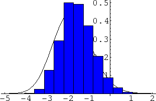
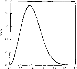
It has been proven that, in the bulk spectrum, the normalized spacings have a limiting distribution as
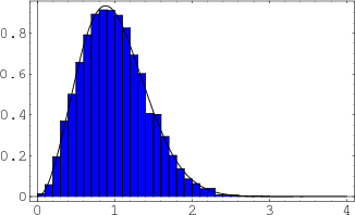
![]() , called the Gaudin distribution. The density of the Gaudin distribution cannot be written in closed form, although it can be computed numerically. In Figure 6, we show a simulation of the normalized spacing distribution for 500 random GUE matrices of size
, called the Gaudin distribution. The density of the Gaudin distribution cannot be written in closed form, although it can be computed numerically. In Figure 6, we show a simulation of the normalized spacing distribution for 500 random GUE matrices of size
![]() We have also superimposed the Gaudin density. We see that the fit is quite good.
We have also superimposed the Gaudin density. We see that the fit is quite good.
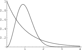
In Figure 7 we compare the Gaudin density with the Poisson density. We note that in the Poisson case, small values are quite probable, while in the normalized spacing case, such values are much less probable. This is sometimes described by saying that the eigenvalues `repulse' one another.
The analog of Montgomery's conjecture for the gaps for the normalized eigenvalues is:
The hypothesis that the zeros of the zeta function and the eigenvalues of GUE matrices have the same pair correlation function is called the GUE hypothesis (or the Montgomery-Odlyzko law). Odlyzko contributed to this hypothesis by calculating a very large number of zeros of the Riemann zeta function and using these to support the GUE Hypothesis. As we have seen earlier in Figure 4, Odlyzko compared the empirical pair correlation for the normalized zeros of the zeta function to the conjectured limiting distribution and found a remarkably good fit.
 |
Odlyzko also compared the limiting distributions for the normalized spacings of the eigenvalues of GUE matrices with the distribution of the normalized spacings of the zeros of the zeta function as shown in Figure 8. We see that the fits again remarkably good and this has led to the hope that the use of the theory of random matrices will lead to a proof of the Riemann hypothesis.
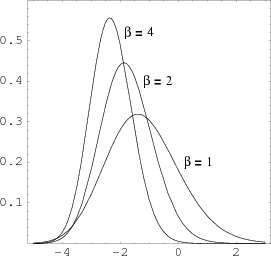
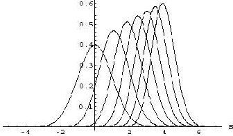
Tracy and Widom [9] showed that the largest eigenvalue, properly normalized, tends to a limiting distribution. These limiting distributions were different for the three possible values of ![]() corresponding to the three different ensembles. Their densities are shown in Figure 9. They are denoted by
corresponding to the three different ensembles. Their densities are shown in Figure 9. They are denoted by ![]() and they are now called Tracy-Widom distributions. As with the Gaudin distribution there is no formula for these densities though they can be computed numerically. These distributions have been found to be the limiting distributions in many different fields and appear to indicate a new central limit theorem.
and they are now called Tracy-Widom distributions. As with the Gaudin distribution there is no formula for these densities though they can be computed numerically. These distributions have been found to be the limiting distributions in many different fields and appear to indicate a new central limit theorem.
Let ![]() be the largest eigenvalue of a random
be the largest eigenvalue of a random ![]() GUE matrix. Then Tracy and Widom proved that
GUE matrix. Then Tracy and Widom proved that
 |
The discovery of these distributions has led Tracy and Widom and others to find these distributions as limiting distributions for phenomena in a number of different areas outside of the study of random matrices. We now discuss two such applications.
Around 1960, Stanislaw Ulam considered the following problem: Given a positive integer ![]() , let
, let ![]() be a random permutation of the integers from 1 to
be a random permutation of the integers from 1 to ![]() . Let
. Let ![]() be the length of the longest increasing subsequence in
be the length of the longest increasing subsequence in ![]() . For example, if
. For example, if
![]() the longest increasing sequence is
the longest increasing sequence is ![]() , so
, so
![]() Ulam asked: what is the average value of
Ulam asked: what is the average value of ![]() ? Based upon Monte Carlo simulations, Ulam conjectured that the average length is asymptotic to
? Based upon Monte Carlo simulations, Ulam conjectured that the average length is asymptotic to ![]() . This conjecture was proven by Vershik and Kerov [6]. Recently the distribution of
. This conjecture was proven by Vershik and Kerov [6]. Recently the distribution of ![]() has been the subject of much research. In particular, Baik, Deift, and Johansson [7] have shown that if
has been the subject of much research. In particular, Baik, Deift, and Johansson [7] have shown that if ![]() is scaled in the appropriate way, then the distribution of
is scaled in the appropriate way, then the distribution of ![]() approaches a limiting distribution as
approaches a limiting distribution as
![]() . More precisely, they show that the random variable
. More precisely, they show that the random variable
Another interesting example is based on a model for the spread of a fire studied by Gravner, Tracy and Widom (GTW) [8]. We imagine a large sheet of paper and a fire starting in the bottom left corner. The fire moves deterministically to the right but also moves up by a random process described next.
We start with a grid of unit squares on the paper. We label the rows
![]() and the columns
and the columns
![]() We represent the spread of the fire by a placing letters H or D in the squares of the grid. We start at
We represent the spread of the fire by a placing letters H or D in the squares of the grid. We start at ![]() with a letter D at (0,0). To get the configuration of the fire at time
with a letter D at (0,0). To get the configuration of the fire at time ![]() we look at the fire in columns 0 to t+1 at time t. If the height of the fire at a column is less than the height of the fire in the column to its left, we add a D to the column. If the height of the fire is greater than or equal to the height of the fire in the column to its left, we toss a coin. If heads comes up we add an H to the height of the column. For column 0 which has no column to the left we always toss a coin to see if we should add an H to this column.
we look at the fire in columns 0 to t+1 at time t. If the height of the fire at a column is less than the height of the fire in the column to its left, we add a D to the column. If the height of the fire is greater than or equal to the height of the fire in the column to its left, we toss a coin. If heads comes up we add an H to the height of the column. For column 0 which has no column to the left we always toss a coin to see if we should add an H to this column.
Let's see in more detail how this works. We start at time 0 and put a D in column 0 and so the height of the fire in this column is 1.
                   t = 0     D
                             0   1   2   3   4   5   6.
At time t = 1 we look at columns 0 and 1 at time 0. The height of the fire in column 1 is less than in column 0 so we add a D to this column. In column 0 we toss a coin. It came up heads so we added an H to the first blank square in this column. Thus for time t = 1 we have:
                   t = 1     H
                             D   D
                             0   1   2   3   4   5   6.
Now at time
                             H   D
                   t = 2     D   D   D
                             0   1   2   3   4   5   6.
Continuing in this way we have:
                                 H
                   t = 3     H   D   D
                             D   D   D   D
                             0   1   2   3   4   5   6

                                 H
                                 H   D
                    t = 4    H   D   D   D
                             D   D   D   D   D
                             0   1   2   3   4   5   6

                                 H   D
                             H   H   D   D
                    t = 5    H   D   D   D   D
                             D   D   D   D   D   D
                             0   1   2   3   4   5   6

                                     H
                                 H   D   D
                    t = 6    H   H   D   D   D
                             H   D   D   D   D   D.
Let ![]() be the height of the fire in column
be the height of the fire in column ![]() after time
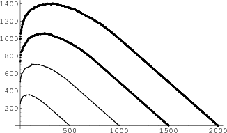
after time ![]() We wrote a Mathematica program to simulate the spread of the fire. We ran the program for t = 500, t = 1000 and t = 2000. In Figure 12 we show plots of the height of the fire,
We wrote a Mathematica program to simulate the spread of the fire. We ran the program for t = 500, t = 1000 and t = 2000. In Figure 12 we show plots of the height of the fire, ![]() , for these three times.
, for these three times.
Note that up to time ![]() the graphs have a curved shape and after
the graphs have a curved shape and after ![]() they seem to follow a straight line. This behavior is completely described by the limiting results obtained by GTW.
they seem to follow a straight line. This behavior is completely described by the limiting results obtained by GTW.
In our simulations we have assumed that the coin that is tossed is a fair coin. The authors consider more generally that the probability that the coin turns up head is ![]() . The authors prove limit theorems for the height of the fire after time
. The authors prove limit theorems for the height of the fire after time ![]() under the assumption that
under the assumption that ![]() and
and
![]() in such a way that their ratio
in such a way that their ratio ![]() is a positive constant
is a positive constant ![]() for
for ![]() . Their limit theorems use two constants,
. Their limit theorems use two constants, ![]() and
and ![]() which depend on
which depend on ![]() and
and ![]() . These constants are:
. These constants are:
![\begin{displaymath}c_2(p,p_c) = (p_c(1-p_c))^{1/6}(p(1-p))^1/2 \left[\left (1+\s...
...rac {p_c}{1-p_c}}- \sqrt{\frac {p}{1-p}}\right )\right ]^{2/3}.\end{displaymath}](img122.png)
The authors prove the following limit theorems showing what happens when the ratio x/t = c is kept fixed with c a positive constant. They have limit theorems for four different ranges for c.
Note that, since it takes ![]() time units for the fire to reach column
time units for the fire to reach column ![]() can be at most
can be at most ![]() . The authors provide the following numerical values of the limiting distribution for negative integers.
. The authors provide the following numerical values of the limiting distribution for negative integers.
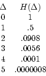
Note again that ![]() can be at most
can be at most ![]() so this says that, in this regime, in the limit, the fire in column x reaches its maximum possible height.
so this says that, in this regime, in the limit, the fire in column x reaches its maximum possible height.
Let's see what these limit theorems would predict for the height of the fire at t = 2000 when p =1/2. The GUE universal regime will apply for
![]() . Here the limiting result in this regime implies that
. Here the limiting result in this regime implies that
![]() should be approximately
should be approximately
![]() . The critical regime applies when x = 1000. Here the limit theorem says that
. The critical regime applies when x = 1000. Here the limit theorem says that
![]() will be approximately 1000. The deterministic regime will apply for
will be approximately 1000. The deterministic regime will apply for
![]() . The limiting theorem for this regime implies that, for
. The limiting theorem for this regime implies that, for ![]() ,
, ![]() is well approximated by the line
is well approximated by the line ![]()
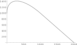
Putting all this together we would predict that for, t = 2000, the limiting curve should be as shown in Figure 13.
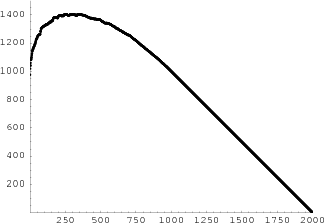
In Figure 14 we show the result of simulating the fire for 2000 time units.
These two graphs are remarkably similar. In fact, if you superimpose them you will not be able to see any difference! Thus the limit results predict the outcome for large t very well.
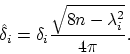
The authors also consider a fourth regime which they call the finite ![]() GUE regime For this regime they fix
GUE regime For this regime they fix ![]() and let
and let
![]() Thus they look for the limiting distribution for the height of the fire in a specific column. For this they prove that
Thus they look for the limiting distribution for the height of the fire in a specific column. For this they prove that
Since for column one we are just tossing coins to determine the height of the fire, we will get the normal distribution as limiting distribution for column 0, and this is ![]()
This document was generated using the LaTeX2HTML translator Version 2002-2-1 (1.70)
Copyright © 1993, 1994, 1995, 1996,
Nikos Drakos,
Computer Based Learning Unit, University of Leeds.
Copyright © 1997, 1998, 1999,
Ross Moore,
Mathematics Department, Macquarie University, Sydney.
The command line arguments were:
latex2html -split 0 -no_math -html_version 3.2 -white -no_transparent part3aug10.tex
The translation was initiated by Peter Kostelec on 2005-04-05