Prepared by J. Laurie Snell, Bill Peterson, Jeanne Albert, and Charles Grinstead, with help from Fuxing Hou and Joan Snell.
We are now using a listserv to send out Chance News. You can sign on or off or change your address at this Chance listserv. This listserv is used only for mailing and not for comments on Chance News. We do appreciate comments and suggestions for new articles. Please send these to:
jlsnell@dartmouth.edu
The current and previous issues of Chance News and other materials for teaching a Chance course are available from the Chance web site.
Chance News is distributed under the GNU General Public License (so-called 'copyleft'). See the end of the newsletter for details.
It is evident that the primes are randomly distributed but, unfortunately we don't know what 'random' means.
R.C. Vaughan
In Chance News 10.10 Dan Rockmore wrote Chapter 1 of our story Chance in the Primes. This story is intended to help our readers understand Peter Sarnak's popular exposition of the Riemann Hypothesis. In Chapter I Dan gave background material to help in understanding Sarnak's history of prime number theory given in the first part of his lecture. This chapter, written by Laurie is a bit of a digression from Sarnak's talk and provides additional examples of how chance has been used in the study of prime numbers. In the the next chapters we Dan will return to Sarnak's talk and explain basic concepts of quantum theory and random matrices and how they are related to a new approach to proving the Riemann Hypothesis.
The prime numbers are a deterministic sequence of numbers and so it is worth thinking about why probability might given insight into the primes.
When our colleague Peter Doyle was a boy he used to go for walks with his friend Jeff Norman using the digits of p to decide which way to go when they came to an intersection -- they had memorized about the first 1000 digits. It might have occurred to them to ask: when they started at Peter's home, what is the probability that we they will eventually return to his home? If they had heard of Polya's theorem that a random walk in one or two dimension will return to its starting point, they might have felt more confident that they would return home even though their walk was not determined by a chance process.
With the introduction of random number generators, we have become quite used to using a deterministic sequence of numbers to illustrate the basic theorems of probability. We could even use the first billion or so digits of p to beautifully illustrate the law of large numbers or the central limit theorem. But with the study of primes, we want to go the other way. We want to use knowledge about a chance process to better understand the primes just the way that Jeff and Peter might have learned something about their walk from Polya's theorem.
Our discussion in this chapter will show ways that people have tried to get new information about the primes by using known theorems or proving new theorems about related chance processes. This is a very tricky business and we start with an example to show that we can easily be tricked if we are not careful.
A probabilistic proof of the Prime Number Theorem?
Here is a way to try to prove the prime number theorem using probability. Recall
that the prime number theorem states that p(x),
the number of primes less than or equal to x, is asymptotically n/log(n). Assume
that we choose a number X at random from 1 to n. Then Prob(X) is prime) = p(x)/n
so we can state the prime number theorem as:
![]()
If X is not prime it must be divisible by a prime less than or equal to sqrt(n). Since every kth number is is divisible by k the probability that X is divisible by k is 1/k. Thus, the probability that X is prime is the probability that it is not divisible by any prime less than or equal to the sqrt(n). For example, the sqrt(200)) = 14.14.. So
Probability X is prime = (1-1/2)(1-1/3)(1-1/5)(1-1/7)(1-1/11)(1-1/13) = .192.
Thus to prove the prime number theorem we must prove that:
where p is a prime number. But Merten proved that:
where g=.57729... is Euler's constant and so
![]()
and so our probabilistic proof gives the wrong answer! We could have already seen that our product formula was wrong by checking our answer for n = 200. Since p(x) = 46, Prob(X is prime) = 46/200 = .23 and not .192 that our product formula gave us. There are two things wrong with our calculation. First, while it is true that half the numbers from 1 to 200 are divisible by 2, it is not true that 1/3 are divisible by 3. The number divisible by 3 in the first 200 numbers is the integer part of 200/3 = 66. Thus only 33% of the first 200 numbers are divisible by 3 rather than 33.333..% we assumed.
Secondly, like our students we have assumed that we can simply multiply probabilities to find the probability that several events are all true. Let's see if the events E = "X is divisible by 2" and F = "X is divisible by 3" are independent events. This is true if n is divisible by 2 and 3. For example, if n = 12, there are 6 numbers divisible by 2, 4 numbers divisible by 3, and 2 numbers divisible by both 2 and 3. Thus P(E) = 1/2, P(F) = 1/3 and P(E and F) = 1/6, so P(E and F) = P(E)P(F) = 1/6 and E and F are independent. However, if n = 13, then P(E) = 6/13, P(F) = 4/13 and P(E and F )= 2/13 which is not equal to P(E)P(F) = 24/169. Thus E and F are not independent.
One might hope that asymptotically these two problems would disappear but Merten's result shows that this is not the case. This is also illustrated by the following exact calculations:
The density of prime numbers.
In an interesting article, "Harold Cramer and the distribution of prime numbers" Scandanavian Actuarial J. 1 (1995), 12-28 ), Andrew Granville writes that Gauss, in a letter to Encke, on Christmas Eve 1947, said:
As a boy I considered the problem of how many primes
there are up to a given point. From my computations, I determined that the density
of primes around x, is about 1/log(x).
What does "the density of primes around x is about 1/log(x)" mean? If p(x) is a density function for a chance experiment, we think of p(x) as the probability that the outcome is in an interval [x, x + Dx] where Dx is small compared to x. But f(x) =1/log(x) is not a probability density since its integral over the positive numbers is infinite. However, we can do something similar to what we do for a probability density.
Let D(x) be a function of x that goes to infinity slower than x, i.e., x + D(x) is asymptotically x. Then we will show that the prime number theorem implies that the proportion of numbers in the interval [x, x + D(x)] that are prime is asymptotically 1/log(x). Thus, the probability that an integer chosen at random in the interval [x, x + D(x)] is prime is approximately 1/log(x).
Recall that the Prime Number theorem states that
![]() .
.
Here p(x) is the number of
primes less than or equal to x. The proportion of numbers in the interval [x,
x + D(x)] that are prime is(p(x
+ D(x)) - p(x))/D(x).
We need to show that the ratio of this to 1/log(D(x))
approach 1 as x approaches infinity. But
as was to be proven.
We illustrate this approximation for D(x) = sqrt(x).
|
n
|
D(x) |
Interval
|
number of primes in the interval.
|
probability that a randomly chosen
integer in the interval is prime
|
approximate probability |
ratio of exact to approximate probability
|
|
100
|
10
|
[100, 110]
|
4
|
.4
|
.217147
|
1.8421
|
|
10,000
|
100
|
[10,000, 10,100]
|
11
|
.11
|
.108574
|
1.01314
|
|
100,000
|
1,000
|
[100,000, 101,000]
|
75
|
.075
|
.0723824
|
1.03616
|
|
1,000,000
|
10,000
|
[1,000,000,1,010,000]
|
551
|
.0551
|
.0542868
|
1.01498
|
|
10,000,000
|
100,000
|
[10,000,000, 10,100,000]
|
4306
|
.04306
|
.0434294
|
.991493
|
|
100,000,000
|
1,000,000
|
[100,000,000, 1,01,000,000]
|
36249
|
.036249
|
0361912
|
1.0016
|
Here is an application of this result. The success of one of the modern encryption methods rests on the fact that it easy to find two 200 digits prime numbers but, given the product of these two numbers, it is extremely difficult to factor this product to recover the two prime factors. We shall explain how this fact is used to obtain a secure method of encryption later. Here we will show why it is easy to find 200 digit primes.
Let x = 10^200 and Dx = sqrt(x) = 10^100. Then we have just shown that, if we choose one of these numbers at random, the probability that it is prime is approximately 1/log(Dx) = .004.. . Thus if we choose 250 such numbers we should expect to get at least one prime number. So this is a practical way to find a 200 digit prime. We used Mathematica to choose 400 random 200-digits numbers and then to test them for primality. We found 2 prime numbers and multiplied them together to obtain the number:
478857666143822033324269962220157253835020621786762268629403225926037628569395
230189709910293445147137522991535640944560209169903096737299891297201537052227
747108164393721763692326209734550472598504487065520874179490318662382292423893
140419161783580414731479843707556332612818564502522206694081650171127530811923
067907784340544294144952881559230521817255464542588707573028382273761890209597.
We will give a year's subscription to Chance Magazine to the first person who tells us what our prime numbers were.
We should confess that we do not have complete confidence that our 200 digit numbers are prime. We identified them using Mathematiac's function PrimeQ to test primality which is known to be accurate only up to 10^16 so could conceivable be wrong for 200 digit numbers. In practice, 200 digit prime numbers used for encryption are chosen by a method that produces numbers called "probably-primes" which are known to be prime with a very high probability. We will discuss this method later.
Cramer's random primes.
Here is a table of the first 225 prime numbers
|
2
|
3
|
5
|
7
|
11
|
13
|
17
|
19
|
23
|
29
|
31
|
37
|
41
|
43
|
47
|
|
53
|
59
|
61
|
67
|
71
|
73
|
79
|
83
|
89
|
97
|
101
|
103
|
107
|
109
|
113
|
|
127
|
131
|
137
|
139
|
149
|
151
|
157
|
163
|
167
|
173
|
179
|
181
|
191
|
193
|
197
|
|
199
|
211
|
223
|
227
|
229
|
233
|
239
|
241
|
251
|
257
|
263
|
269
|
271
|
277
|
281
|
|
283
|
293
|
307
|
311
|
313
|
317
|
331
|
337
|
347
|
349
|
353
|
359
|
367
|
373
|
379
|
|
383
|
389
|
397
|
401
|
409
|
419
|
421
|
431
|
433
|
439
|
443
|
449
|
457
|
461
|
463
|
|
467
|
479
|
487
|
491
|
499
|
503
|
509
|
521
|
523
|
541
|
547
|
557
|
563
|
569
|
571
|
|
577
|
587
|
593
|
599
|
601
|
607
|
613
|
617
|
619
|
631
|
641
|
643
|
647
|
653
|
659
|
|
661
|
673
|
677
|
683
|
691
|
701
|
709
|
719
|
727
|
733
|
739
|
743
|
751
|
757
|
761
|
|
769
|
773
|
787
|
797
|
809
|
811
|
821
|
823
|
827
|
829
|
839
|
853
|
857
|
859
|
863
|
|
877
|
881
|
883
|
887
|
907
|
911
|
919
|
929
|
937
|
941
|
947
|
953
|
967
|
971
|
977
|
|
983
|
991
|
997
|
1009
|
1013
|
1019
|
1021
|
1031
|
1033
|
1039
|
1049
|
1051
|
1061
|
1063
|
1069
|
|
1087
|
1091
|
1093
|
1097
|
1103
|
1109
|
1117
|
1123
|
1129
|
1151
|
1153
|
1163
|
1171
|
1181
|
1187
|
|
1193
|
1201
|
1213
|
1217
|
1223
|
1229
|
1231
|
1237
|
1249
|
1259
|
1277
|
1279
|
1283
|
1289
|
1291
|
|
1297
|
1301
|
1303
|
1307
|
1319
|
1321
|
1327
|
1361
|
1367
|
1373
|
1381
|
1399
|
1409
|
1423
|
1427
|
In his lecture
on the Riemann Hypothesis, Jeffrey Vaaler pointed out that it is hard to see
any pattern in these numbers. This apparent randomness in the distribution of
prime numbers has suggested to some that, even though the primes are a deterministic
sequence of numbers, we might learn about their distribution by assuming that
they have, in fact, been produced randomly. An interesting example of this approach
appeared in the 1936 paper of Harold Cramer "On the order of magnitude
of the difference between consecutive prime numbers," Acta. Arithmetic,
2, 23-46. Of course, we know Cramer from his work in probability and
statistics and, in particular, from his classic book "Mathematical Methods
of Statistics" which is still in print. However, his thesis and early papers,
were in prime number theory.
Cramer considered the following very simple chance process to investigate questions
about the prime numbers. He imagined a sequence of urns U(n) for n = 1,2,...
. He puts black and white balls in the urns in such a way that if he chooses
a ball at random from the kth urn, it will be white with probability 1/log(k).
Then he chooses 1 ball from each urn and calls the numbers for which the balls
were white "random primes." Note that, unlike true primes, random
primes can be even numbers. In his paper that we mentioned above, Granville
describes a number of results that Cramer proved for his random primes that
led to a better understanding of the true primes. We shall illustrate this in
terms of a result that led to a conjecture for the real primes that has not
yet been settled.
In his earlier research, Cramer studied the gaps that occur between prime numbers. A gap in the sequence of prime numbers is the difference of two successive primes. Such gaps can be arbitrarily large. We can see this as follows: 4! = 4x3x2x1. Thus the integers 4!-2, 4!-3, 4!-4 are not prime so we have a gap of at least 3. More generally, n! - j are not prime for j = 2 to n so, for any n, there is a gap of at least n-1. We say that a gap is a "record gap" if, as we go through the sequence of primes, this gap is larger than any previous gap. For example, for the first 10 primes 2, 3 ,5 ,7, 9, 11, 13, 17, 19, 23, 29 the gaps are 1, 2, 2, 2, 2 2, 4 ,2, 4, 6. So the first four record gaps are 1, 2, 4, and 6. Cramer, using the Borel-Cantelli lemma, proved that for these random primes the nth record gap is asymptotically the (log(p))^2 where p is the starting prime for the gap.
We simulated Cramer's chance process to obtain a sequence of a hundred million pseudo-random primes. In this sequence there were 19 record gaps. Here is a graph of the ratios of these record gaps, normalized by dividing by the square of the initial prime in the gap. According to Cramer's conjecture this graph should approach 1.
Let's compare this with a with a graph of the record gaps for
real prime numbers. Record gaps are maintained by Thomas
Nicely. There have been 63 record gaps found todate, the largest of which
is 1132 which starts at the prime 1693182318746371. The (log(1693182318746371))^2
= 1229.58 so this record gap normalized is 1132/1229.58 = .92 which is close
to the limiting ratio of 1 as Cramer conjectured. Here is a graph of the 63
normalized record gaps.
Note that the evidence for Cramer's conjecture looks more convincing for the true primes, for which it has not been proven, than for the random primes where it has been proven.
What about small gaps? Except for the first two prime numbers (2,3) the smallest gap that could occur is 2. When this occurs we say we have a "twin prime". One of the most famous unsolved problems in prime number theory is: are there infinitely many twin primes? Let's see if this is true for Cramer's random primes. Since random primes can be even, it might be more natural to consider "twin primes" as pairs n, n+1 where n and n+1 are random primes. Then, since the events "n is a random prime" and "n+1 is a random prime" are independent, the probability that the pair n,n+1 are twin primes is 1/log(n)log(n+1). Since the sum of these probabilities diverges, the Borel-Cantelli lemma implies that, with probability 1, we will have infinitely many twin random primes. Note that there also will be infinitely many pairs of the form n, n +k for any integer k.
The Eratosthenes sieve.
A more sophisticated definition of random primes was introduced later by the philosopher David Hawkins (Hawkins, D. 1958. Mathematical sieves. Scientific American 199(December):105). His method of generating random primes was suggested by a technique introduced by Eratosthenes of Cyrene (275-194 BC) called the "Eratoshenes Sieve."
The Eratosthenes sieve is a way to find all the primes less than or equal to n. We illustrate how the sieve works for n = 200 using an applet that you can find here.
If p is a prime between 1 and n it must be divisible by a prime less than or equal to the square root of n. For n = 200 the Eratosthenes sieve proceeds by successively removing numbers divisible by the primes less than the sqrt(200) = 14.1, i.e., by the primes 2,3,5,7,11,13.
We start with a table of the integers from 2 to 200.
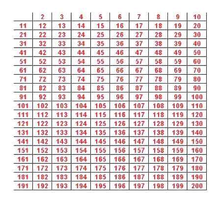
We then proceed to "sieve out" all the numbers divisible by the first prime number 2.
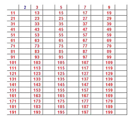
Next we sieve out all numbers greater than 2 that are divisible by 3 obtaining:
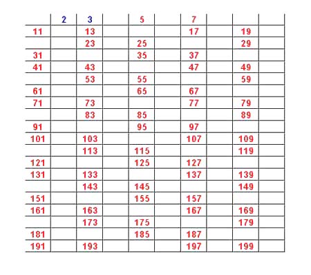
We continue sieving out divisors of 5,7,11, and 13 and the resulting numbers are the primes in the first 200 numbers.
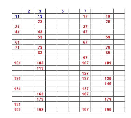
We see that there are 46 such prime numbers.
The Eratotshenes Sieve suggested to David Hawkins a new way to generate random primes. He defines his process by a probability sieve. Start with the integers beginning with 2:
2, 3, 4, 5, 6, 7, 8, 9, 10, 11, 12, 13, 14, 15, 16, 17, 18, 19, 20, 21 ,22, 23,... .
Now throw out each number with probability 1/2. Suppose this leaves us with
3, 4, 5, 7, 10, 11, 13, 14, 17, 18, 19, 23,... .
Then the first number 3 is the first random prime. Now go through this sequence throwing out each number greater than 3 with probability 1/3 leaving for example,
3, 5,7,10,11... .
Then 5 is the next prime number. Next throw out each number greater than 5 with probability 1/5. Continue in this way to obtain a sequence of random primes.
Of course, it is easy to simulate random primes. Here are the primes less than or equal to 1000 that resulted from one such simulation:
|
2
|
4
|
6
|
12
|
16
|
19
|
26
|
28
|
30
|
34
|
37
|
41
|
43
|
|
44
|
52
|
57
|
60
|
61
|
68
|
70
|
75
|
81
|
83
|
88
|
89
|
91
|
|
94
|
100
|
103
|
105
|
107
|
111
|
117
|
130
|
131
|
134
|
135
|
137
|
146
|
|
152
|
157
|
163
|
172
|
173
|
174
|
175
|
176
|
193
|
198
|
205
|
208
|
211
|
|
215
|
218
|
222
|
223
|
228
|
241
|
256
|
257
|
263
|
269
|
271
|
287
|
290
|
|
291
|
298
|
302
|
313
|
322
|
324
|
352
|
358
|
377
|
380
|
382
|
384
|
389
|
|
398
|
412
|
420
|
429
|
431
|
433
|
435
|
444
|
451
|
474
|
485
|
492
|
495
|
|
497
|
500
|
529
|
546
|
562
|
564
|
568
|
571
|
583
|
599
|
602
|
603
|
610
|
|
625
|
626
|
629
|
640
|
644
|
661
|
663
|
669
|
681
|
693
|
699
|
706
|
709
|
|
719
|
733
|
738
|
742
|
752
|
767
|
782
|
792
|
802
|
810
|
814
|
839
|
840
|
|
861
|
869
|
894
|
905
|
907
|
910
|
911
|
912
|
919
|
923
|
924
|
927
|
938
|
|
940
|
962
|
966
|
970
|
981
|
982
|
Hawkins and others proved a number of theorems for Hawkins' random primes similar to well- known theorems about the true prime numbers. For example,Wunderlich showed that, with probability one, Hawkins' random primes satisfy the prime number theorem. That is, the number of random primes less than n is asymptotically n/log(n). In our simulation there are 149 random primes less than 1000. The prime number theorem would predict 1000/log(1000) = 144.77 which is closer than the result for real primes but, of course, both estimates are meant to be for large n.
Since, for random primes, even numbers can be prime, a natural "twin prime" theorem would be that there are infinitely many pairs of random primes of the form k, k+1. Wunderlich showed that, with probability one, Hawkins' random primes have infinitely many twin primes, i.e., infinitely many pairs k, k+1. He also showed that, with probability one, the number of such twin primes less than n is asymptotically n/(log n)^2.
We can get a heuristic estimate for this same result for true primes by assuming that the occurrences of a twin prime at n and n+2 are independent. Then, using the prime number theorem, the probability that n, n+ 2 for odd n is a twin prime is approximately 1/log(n)xlog(n+2). Thus we would expect the number of twin primes less than n, p2(x), to be asymptotically n/(log n)^2 . Hardy and Wright gave this probabilistic argument but then gave an improved estimate:
where c = 1.320... . This estimate is remarkably good. From this
web site we find an interesting discussion of twin primes and the following
table comparing the Hardy Wright estimate with the true numbers of twin primes
for values of n for which the number of twin primes are known todate:
|
n
|
Twin primes < n
|
Hardy Wright estimate
|
Relative error
|
| 10 | 2 | 5 | 150 |
| 100 | 8 | 14 | 75 |
| 1000 | 35 | 46 | 31.43 |
| 10000 | 205 | 214 | 4.39 |
| 100000 | 1124 | 1249 | 11.12 |
| 1000000 | 8169 | 8248 | .97 |
| 10000000 | 58980 | 58754 | -.38 |
| 100000000 | 440312 | 440368 | .013 |
| 1000000000 | 3424506 | 3425308 | .023 |
| 10000000000 | 27412679 | 27411417 | -.0046 |
| 100000000000 | 224376048 | 224368865 | -.0032 |
| 1000000000000 | 1870585220 | 1870559867 | -.0013 |
| 10000000000000 | 15834664872 | 15834598305 | -.00042 |
| 100000000000000 | 135780321665 | 135780264894 | -.000042 |
| 1000000000000000 | 1177209242304 | 1177208491861 | -.0000064 |
| 5000000000000000 | 5357875276068 | 5357873955333 | -.0000025 |
Of course, it is natural to ask if there is a chance process that can shed light on the truth or falsity of the Rieman Hypotheses. We will illustrate this in terms of an approach suggested by von Sternach in 1896.
Recall that for the s > 1 the zeta(s) can be expressed as the infinite series
The reciprocal of the zeta function, is given by
where m(n) is the Moebius function defined by m(n) = 0 if n if is divisible by a square and otherwise m(n) = 1 if the number of prime factors of n is even and -1 if the number of prime factors is odd.
Here are the values of m(n) for n
= 1 to 20
| n | 1 | 2 | 3 | 4 | 5 | 6 | 7 | 8 | 9 | 10 | 11 | 12 | 13 | 14 | 15 | 16 | 17 | 18 | 19 | 20 |
| m(n) | 1 | -1 | -1 | 0 | -1 | 1 | -1 | 0 | 0 | 1 | -1 | 0 | -1 | 1 | 1 | 0 | -1 | 0 | -1 | 0 |
These digits look rather random and might be thought of as the record of a drunkard
who walks down a street, and at the nth corner either decides to rest (m(n)
= 0), to go ahead one block (m(n) = 1) or go back
one block (m(n) = -1). We shall call such a walk
a "prime walk." Of course this is similar to the "random"
walk that Jeff and Peter took using the digits of p.
We denote by g(n) the sum of the first n values of the Moebius function. Thus g(1) = 1, g(2) = 0, g(3) = -1, g(4) = -1, g(5) = -2, g(6) = -1 etc. Then g(n) tells us after time n how far our prime walker is from home.
The first person to suggest comparing the prime walk with a random walk was von Sternach in 1896 and you should click here and read Peter Doyle's two page translation of his description of this random walk before going on with our discussion.
Note that von Sternach calculated the first 150,000 values of g(n).(How would you like to compute 150,000 values of g(n) without a modern computer?) He found that m(n) was non-zero about a proportion 6/p^2 = .608 of the times.. The proportion of 1's and -1's was about the same. Thus for his random walk Sternach chose the probability of a 0 to be 1-6/p^2 = .392...and the probabilities for a 1 and for a -1 to be 3/p^2 = .30399... to make the sum 1.
We will make the same choices. But first we will show that Sternach's estimate holds for the limiting proportion of 0's in the prime walk. Let's count the the number of integers k between 1 to n for which the the m(k) is -1 or 1. This will be the case if k is not divisible by the square of a prime number--i.e., is square-free. The fraction of such numbers will be the probability that a randomly chosen integer X between 1 and n is square-free. Using the same probability argument we used for our probabilistic proof of the prime number theorem we estimate the probability that a random number from 1 to n is square free by:
Recall that the product formula for zeta(s) for s > 1 is:
Thus the probability that X is square free should approach 1/z(2) = 6/p^2 = .607927. But we have again assumed independence and that got us in trouble trying to give a probabilistic proof of the prime number theorem. However, as the following computation shows this time the it appears to work.
We can also compute the exact proportion of square free numbers but not for such large n. Here is a comparison of the exact values and the values obtained by our product formula for values of n up to a million.
The true probability that a random number X from 1 to n is square free does appear to approach 6/p^2 as predicted by our by our product formula. The reason that this approximation works here and did not for the prime number theorem, is probably because for the prime number theorem we were trying to estimate the probability that X is prime. But this probability approaches 0 and n tends to infinity. The probability that a random number is square-free approaches a non-zero limit.
Thus, we have convinced ourselves that Sternach was correct in his choice for the probability of a 0. This will determine the probabilities for -1 and 1 if these asymptotic values are equal. Evidently this is true but hard to prove, being equivalent to the prime number theorem! Of course we can also check this claim by computing these proportions for large values of n. Here are the results of such a computation.
| N | Proportion. of -1's | Proportion of 0's | Proportion. of 1's |
| 10 | .4 | .3 | .3 |
| 100 | .30 | .39 | .31 |
| 1,000 | .303 | .392 | .305 |
| 10,000 | .3053 | .3917 | .3030 |
| 100,000 | .30421 | .39206 | .30373 |
| 1,000,000 | .303857 | .392074 | .304069 |
| 10,000,000 | .3039127 | .3920709 | .3040164 |
| 100,000,000 | .30395383 | .39207306 | .30397311 |
| 1,000,000,000 | .303963673 | .392072876 | .303963452 |
| Limiting value | .3039635509.. | .3920728981 | .30396355092.. |
These computations are pretty convincing.
Now we can apply standard probability theorems to our random walk..
The Riemann Hypothesis would be true if one could prove that the lim sup |g(n)| is less than than cxn^(1/2+e) for positive constants c and e -- see Edwards p. 261. That is, if we could prove that our prime walker would not stray to far from home. The iterated logarithm assures us that this is true with probability one for our random walk. Thus, if this is a good model for the behavior of the values of g(n). we can consider this as evidence that the prime number theorem is true.
Sternach included a beautiful graph of 1500,00 values of g(n) that extended over 4 folded pages. He included graphs of sqrt(n) and - sqrt(n) and remarked that the graph of g(n) never got even half way up to these curves. He commented that "if a conjecture is indicated it would be that |g(n)| < sqrt(n) for all n". However, Odlyzko and Riele proved in 1985 that there are infinitely many values of n for which g(n) > 1.06 sqrt(n), though they did not believe that such an example would be found for x < 10^20 or possibly even 10^30. They concluded that they did not believe that there would be any c such that |g(n)| < c sqrt(n) for all n. Of course, this is also suggested by the random walk model. But is the random walk model a good model for g(n)?
Sternach's graph was too big for us to handle, but with modern computers we can make graphs for the first million steps in the prime walk. Also Sternach could not simulate his random walk since he would have to have rolled his die 150,000 times! Here are graphs of the prime walk (the upper picture) and a random walk (the bottom picture).
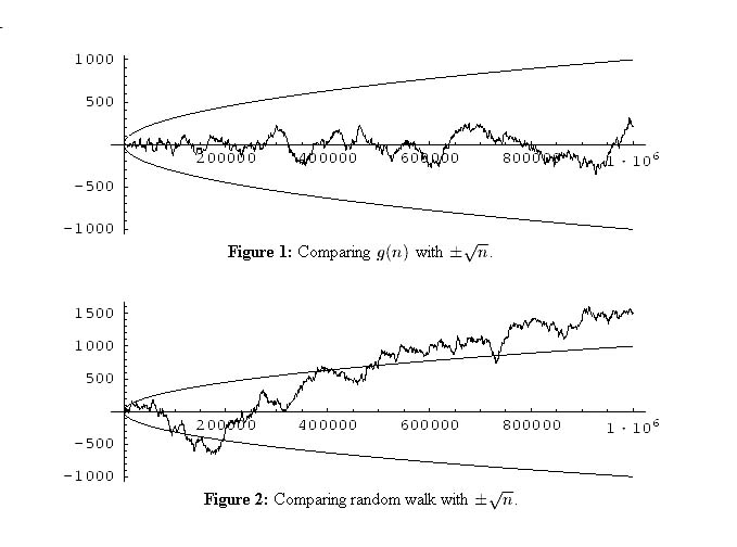
We note that the graphs look quite different which suggests that our prime walk does not behave like a typical sequence in our random walk. There is significantly less variation in the prime walk and it appears to be a kind of oscillatory behavior. The smaller variation was also suggested by Sternach.
Peter Kostelec computed the first first trillion values of g(n). Here is a plot of g(n)/sqrt(n) for a sample of size 8192 chosen uniformly on a logarithmic scale from n = 10^2 to n = 10^12.
If Sternach had just computed to a trillion he would have found that his conjecture that |g(n)| < sqrt(n). is still o.k. However, in this range there are values where g(n) > 1/2sqrt(n) and less than -1/2sqrt(n).
We estimated what the variation should be for a stochastic model for the g(n)'s as follows. We chose a sample of size 10,000 on a log scale of the first billion values of g(n) and normalized the values of g(n) at these points by dividing by sqrt(n). The mean of these normalized values was -.0244452 and the standard deviation .176032.
For the random walk model each step has expected value 0, variance 6/p^2 = .6079.. and standard deviaiton .7796.. So the sum of the steps normlized by dividing by sqrt(n) had mean 0 and standard deviation .7796. Thus the random walk model is certainly not a good way to model g(n).
We also looked at the g(n)/sqrt(n) for our sample. Here is a histogram of these values with a normal plot superimposed.
The fit looks pretty good but this is a good example where you can see that the fit very much depends on the bin sizes you choose.
Peter Doyle also pointed out that it is to be expected that there should be less variation in the prime graph because of known constraints on the values of g(n). For example
![]()
Here when g(n)/i is not an integer we mean the largest integer less than g(n)/i. Here is an example of this relation.
| n | 1 | 2 | 3 | 4 | 5 | 6 | 7 | 8 | 9 | 10 |
| m(n) | 1 | -1 | -1 | 0 | -1 | 1 | -1 | 0 | 0 | 1 |
| g(n) | 1 | 0 | -1 | -1 | -2 | -1 | -2 | -2 | -2 | -1 |
| g(r(10/n)) | -1 | -2 | -1 | 0 | 0 | 1 | 1 | 1 | 1 | 1 |
If we add the values of g(n) for 1` = 1 to 10 we do get 1.
Thus the prime walker must walk in such a way that this restriction is always satisfied whereas our random walker can wander as he pleases.
Our conclusion from all this is that Sternach's random walk is not a good model for the values of the moebius function. but perhaps the process of trying to make it a better random walk will help in understanding why the prime walk really can't wander too far from home.
If we could explain the oscillatory behavior, perhaps we would understand why people talk about the music of the primes.
We thank Peter Kostelec and Charles Grinstead for the Mathematica computations and graph used in this discussion.
Finally we consider an example of the use of probability in the study of prime numbers which has nothing to do with the Riemann Hypothesis but is an example of chance in the primes that has a more obvious application to our daily life. This is the problem of encrypting messages. The problem of encoding messages has a long history and you can read about this here.
We shall discuss this topic in terms of a very simple problem. Alice wants to send Bob his grade in such a way that if someone reads Bob's e-mail they will not be able to determine his grade. She gives grades A,B,C,D,E, or F and wants to code them before sending them to her students. A simple method, that goes back to the way Caesar communicated with his troops, is to encode each letter as a different letter. For example, encode each letter as the letter 3 positions further along in the alphabet, starting at A again when F is reached. If Bob got an A she would send him a D, if he got a B she would send him an E, etc. The amount of the "shift" (in this case it is 3) acts as a "key" to the code and the way to assign the letters using this key is called the "codebook". Thus Alice's key is 3 and her "codebook" is
A B C D E F
D E F A B C.
D E F A B C
A B C D E F
Thus if Alice sends Bob an E he will decode it as a B.
Henry is intercepting the student's mail and wants to decode the grades. In other words he wants to know what Alice has used for a key. Well, if Henry intercepts the grades of everyone (or even a reasonable fraction of the class), then Henry could almost surely figure out the shift by looking at the distribution of the grades that he intercepted and then shift the coded sequence back to make it look more reasonable. (Presumably, in a big class the grade distribution should be bell-curve like with a median around C, assuming no grade inflation!) Having done this he would probably recognize Alice's scheme of just shifting the grades.
The problem of the enemy being able to determine the key by intercepting messages has haunted those who used codes for centuries. The story of the breaking of the German enigma code used in world war II is a fascinating story which you can read about here.
The recognition that it would be easy for internet messages to be intercepted led to the development of coding methods that would make it difficult to decode the message sent, even if the encoded messages were intercepted. An example of this is the RSA code named after its authors Ronald Rivest, Adi Shamir, and Leonard Adleman. We will explain this method for coding messages.
We illustrate the RSA method using our example of Alice sending a grade to Bob. The RSA method is a bit complicated, but fortunately Cary Sullivan and Rummy Makmur have provided here an applet to show how it works. We shall follow this applet in our explanation.
We start by choosing two prime numbers, p and q, and computing their product n = pq. To keep things simple, the applet allows you to pick only small numbers for p and q but, in the actual application of the RSA method, p and q are chosen to be large primes with about 200 digits so that n has about 400 digits. The reason for this is that we are going to want the whole world to know n but not p and q. This will work because there is no known method to factor 400-digit numbers in a reasonable amount of time. Also, our RSA encryption method changes a message into a number m and will only work if m < n. So unless n is large we are limited in the number of different messages we can send at one time.
Responding to the applet we choose the two primes p= 7 and q = 11. Then n = pq = 77. Next we use the Euler function f(n) whose value is the number of numbers less than or equal to x that are relatively prime to n. (Two numbers are relatively prime if they have no common factors). When n is the product of two prime numbers p,q, f(n) = (p-1)x(q-1) since there are q multiples of p and p multiples of q that are less than or equal to pq. And in each of these sets of multiples the number pq is included, so there are exactly p + q -1 multiples of either p or q less than or equal to pq. Or pq - p - q +1 = (p-1)(q-1) numbers relatively prime to pq. Thus,
f(n) = f(7x11) = 6x10= 60.
Next, the applet finds a number e which is relatively prime to f(n). It chooses the smallest such number which is 7. The number e is called the "exponential key." In mod n arithmetic, x has a multiplicative inverse y if xy =1 mod n. (Recall that x mod n is the remainder when n is divided by x). To have such an inverse, x and n must be relatively prime. Since e and f(n) are relatively prime, e has an inverse mod(f(n)) which we denote by d. The applet finds that d = 43. To check this we note that exd = 7x43 = 301 = 1 mod 60. The numbers n and e are called "public keys" and can be made publicly available. The number d is called the "private key" and available only to Bob to decode the message from Alice.
Bob's grade was a B. Alice uses numbers to represent the grades with A = 1, B = 2, etc., so she wants to send the message m = 2.
Alice encrypts her message m as c = m^e mod n. Thus c = 2^27 mod 77 = 51.
Then since d is the mod n inverse of e, ed = 1 mod n. Thus Bob can determine m by computing c^d mod n. This works because
c^d mod n = (m^e)^d mod n = m^(ed) mod n = m mod n = m.
Here we have used that m < n.
Well, we still have not mentioned chance. Chance comes in when we try to choose the 200-digit prime numbers p and q. As we have remarked earlier, standard tests for primality such as the Mathematica's function PrimeQ cannot handle numbers this big with a guaranteed accuracy. It turns out there is a simple method of determining numbers with about 200 digits which have an extremely high probability of being random. The method for doing is suggested by a theorem of Fermat.
Fermat's (Little) Theorem: If p is a prime and if a is any integer, then a^p = a mod p
A number p for which a^p = a (mod p) is called a "probable-prime". By Fermat's theorem every prime is a pseudo-prime. However not every probable-prime is prime. But if we choose a probable-prime at random it is very likely to be a prime. Just how likely has been determined by Su Hee Kim and Carl Pomerance. They showed, for example, that if you pick a random 200-digit probable-prime the probability that n is not prime is less than 00000000000000000000000000385. You can find more precisely what random means here
It is natural to ask how hard it is to test if a 200-digit number x is a probable-prime, is prime. Suppose you are using base 2. Then we have to see if 2^(x-1) = 1 mod x. Fortunately it is practical to raise 2 to such a high power by writing it as a product of smaller powers of 2. This is called the method of repeated squaring.
Well, we hope this has given some idea of how chance has been used in the study of the primes. In our future chapters we shall show how chance is playing a role in one of the current attempts to prove the Riemann Hypothesis.