www.google.com

Prepared by J. Laurie Snell, Bill Peterson, Jeanne Albert, and Charles Grinstead, with help from Fuxing Hou and Joan Snell.

We are now using a listserv to send out notification that a new issue of Chance News has been posted on the Chance website. You can sign on or off or change your e-mail address at this Chance listserv. This listserv is used only for mailing and not for comments on Chance News. We do appreciate comments and suggestions for new articles. Please send these to:

The current and previous issues of Chance News and other materials for teaching a Chance course are available from the Chance web site.

Chance News is distributed under the GNU General Public License (so-called 'copyleft'). See the end of the newsletter for details.

This is a special issue of Chance News. It includes only one item which is a story 'The Chance of a Prime'. The more traditional Chance News will be sent out soon.

In 1998 the Mathematical Sciences Research Institute in Berkeley, California had a three-day conference on Mathematics and the Media. The purpose of this conference was to bring together science writers and mathematicians to discuss ways to better inform the public about mathematics and new discoveries in mathematics. As part of the conference, they asked Peter Sarnak, from Princeton University, to talk about new results in mathematics that he felt the science writers might like to write about. He chose as his topic "The Riemann Hypothesis." This is generally considered the most famous unsolved problem in mathematics and is the major focus of Sarnak's research.

In his talk, Sarnak described some fascinating new connections between the Riemann Hypothesis, physics and random matrices. He used only mathematics that one would meet in calculus and linear algebra. Sarnak's lecture, and a discussion of his talk by the science writers, can be found here under "Mathematics for the Media". (Readers might also enjoy the lecture by Larry Gonick, author of "The Cartoon Guide to Statistics.")

Unfortunately, the discussion of Sarnak's talk by the science writers revealed that most of them were completely lost. The first science writer commenting on the talk said that she felt the way she had at a party with German friends. Her friends would try to speak English for a while but would lapse into and out of German resulting in her understanding very little of the conversation.

Even though Sarnak's talk was not a great experience for most of the science writers, it was an excellent expository talk given by a great mathematician. Our own enjoyment of this talk suggested to us that readers of Chance News would also enjoy it. However, we felt that it would help to have some written commentary to go with the video. Our colleague Dan Rockmore offered to provide such a commentary for us. Dan's first installment, presented below, is related to to the first half of Sarnak's talk dealing with properties of prime numbers and history of the Riemann Hypothesis. In future issues of Chance News Dan will provide commentaries related to the second half of Sarnak's talk in which he explains the connection between the Riemann Hypothesis and physics through random matrices.

Another interested popular talk on the Riemann Hypothesis was given recently be Jeff Laaler at the University of Texas. The Clay Mathematics Institute has offered million dollar prizes for solutions of seven famous outstanding problems in mathematics. One of these problems is the Riemann Hypothesis. The University of Texas mathematics department had a series of Millennium Lectures for the general public with a lecture on each of the seven problems. Jeff gave the lecture on the Riemann Hypothesis. The original video of this lecture was hard to follow since the slides were difficult to read. The Clay Institute provided us with the original tape and the slides and we have put them on the Chance Lecture series in our format developed for our Chance Lectures by photographer Bob Drake that makes it easy to read the slides. You can find Vaaler's lecture at the Chance Lecture Series under "Other Lectures". You can skip most of the introduction by starting at 6 minutes into the video.

To watch these videos you will need the free RealOne Player. which you can obtain here. Finding the free player might seem like a hide and seek game but keep on the free path and you will succeed. You will also need the real player plug-in which comes with recent versions of Real Player. Finally, you will need a connection to the internet which is at true 56 Kbps or faster.

We encourage you to read Dan's commentary from the web before printing it in order to see the wonderful interactive graphics that our colleague Peter Kostelec provided for us. We suggest reading Dan's commentary first, then watching Jeff Laaler's talk and then Sarnak's talk for the final word. You will then be in a position to fully appreciated the news and the movie when this famous problem is finally solved.

HERE IS EPISODE ONE!

Chance in the Primes
Dan Rockmore

We hardly ever think of the good old natural numbers as a place for chance or randomness. Much of mathematics may seem inscrutable, but the numbers $1,2,3,\dots$ spill out, known and familiar, grains making up a mathematical salt of the earth. Nevertheless, the understood aspect of the natural numbers is their additive structure. Getting from one number to another by addition or subtraction poses no mysteries. It is only when we start to think of things multiplicatively that the trouble starts and the surprises enter. In a recent MSRI lecture, Sarnak discusses the ways in which probability and statistics, chance, are helping unravel some of the prime mysteries.

The prime numbers are the basic multiplicative building blocks and there is a great deal of work still ongoing to understand the way in which they are distributed among the natural numbers. As you list them, they seem to fall by chance: 2,3,5,7,11,13,.... Since the time of Euclid we have known that there are an infinite number of primes. His proof is easy to restate. Given any finite collection of primes $p_1,\dots,p_n$ then the number $p_1\times...\times p_n + 1$ is not divisible by any of $p_1,\dots,p_n$ , so must be divisible by primes not among this set. So, given any finite set of primes, this produces a different prime, so no finite set of primes can be complete, so there must be an infinite number.

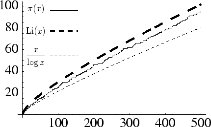
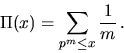
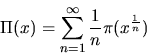
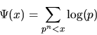
Knowing that there are an infinite number is just the beginning; the next step is to quantify this. More precisely, we define a function

$\pi(x) =$ the number of primes less than or equal to ,

and we study the asymptotics of this function. Based on extensive calculation, Gauss first conjectured and ultimately de Vallee Poisson and Hadamard (1896) proved the "Prime Number Theorem"

$\begin{displaymath}\pi(x) \sim {x\over {\log x}}\end{displaymath}$

that is,

$\begin{displaymath}\lim_{x\rightarrow \infty} {\pi(x) \log x \over x} \rightarrow 1\end{displaymath}$

In fact, Gauss had conjectured (and it implies the Prime Number Theorem) a more precise estimate, that

$\begin{displaymath}\pi(x) \sim Li(x)\end{displaymath}$

where

is the logarithmic integral of

$\begin{displaymath}Li(x) = \int_2^x {dt\over \log t}\end{displaymath}$

As an aside, the comparison of $\pi (x)$ and is the source of one of the largest numbers ever written in a math paper. It is known that is not always greater than $\pi (x)$ , but the first place where it will happen may be around $10^{320}$ .

**Figure 1:** Comparing $\pi (x)$ , Li(x), and $x\over{\log x}$ .
$\begin{figure}\begin{center} \epsfig{figure=threePlotsAll.eps,width=0.8\textwidth}\end{center}\end{figure}$

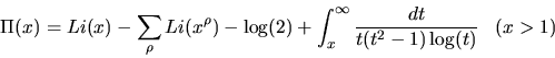
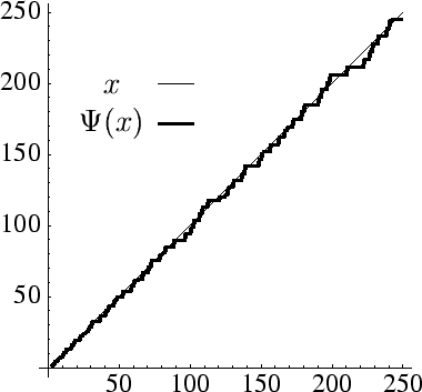
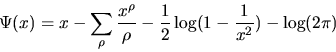
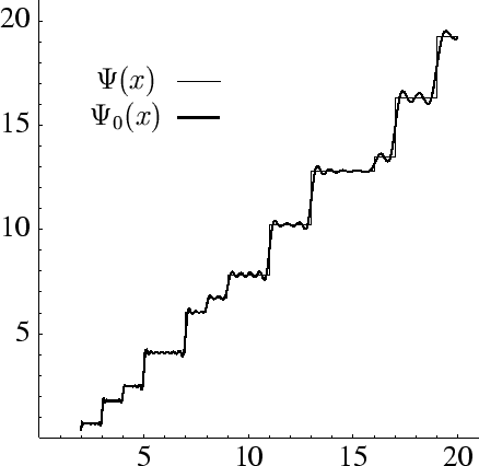
Now, asymptotics are ok, but what is of interest is in getting the estimate as right as can be. That is, we'd like to be able to write that

$\begin{displaymath}\pi(x) = Li(x) + E(x)\end{displaymath}$

where

is the error term in this estimate. Understanding this error term is one of the reasons behind studying "The Riemann Hypothesis". This is a conjecture concerning the behavior of a complex function called the Riemann zeta function, and in particular, understanding the statistical nature of the arguments for which this function is equal to zero, the "zeros" of the zeta function, a lively area at the intersection of number theory, mathematical physics, probability and statistics. Riemann's zeta function, $\zeta(s)$ , for $s = \sigma + i t$ for $i = \sqrt{-1}$ , is the slight generalization to a complex function of a real function first cooked up by the Swiss mathematician Euler. It is defined as

$\begin{displaymath}\zeta(s) = \sum_{n=1}^\infty {1\over {n^{s}}}\end{displaymath}$

For

we get the well-known divergent harmonic series, and for

, the less well-known, but still interesting fact (due to Euler) that $\zeta(2) = {\pi^2\over 6}$ .
One obvious connection to the primes is through Euler's product formula

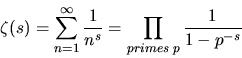
$\begin{displaymath}\zeta(s) = \sum_{n=1}^\infty {1\over {n^{s}}} = \prod_{primes \; p}{1\over{1-p^{-s}}}\end{displaymath}$

The formula results from expanding each of the factors on the right

$\begin{displaymath}{1\over{1-p^{-s}}}= {1 + {1\over{p^s}}}+ {1\over{(p^2)^s}}+{1\over{(p^3)^s}}+\ldots \end{displaymath}$

and noting that their product is a sum of terms of the form

$\begin{displaymath}1\over{{(p_1^{n_1}}{p_2^{n_2}}\cdots p_r^{n_r})^s}\end{displaymath}$

where ${p_1},\ldots {p_n}$ are distinct primes and ${n_1},\ldots {n_r}$ are natural numbers. Then use the Fundamental Theorem of Arithmetic which states that all natural numbers have a unique factorization into prime powers.

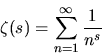
Riemann's great contribution was in linking the zeros of the zeta function to the asymptotics of $\pi (x)$ . He first was able to show that even though $\zeta(1)$ diverges to infinity, the zeta function did have a consistent definition at all other points in the complex plane. In other words, while it is easy to see that $\zeta(s)$ makes sense for any with real part greater than , he was able to find an analytic continuation of $\zeta(s)$ to the entire complex plane, outside of a singularity at . Part of this work was the discovery of the "functional equation" which relates the values of $\zeta(s)$ to the those of $\zeta(1-s)$ - like some funny sort of mirror symmetry about the line .
The functional equation immediately shows that there are some easy to find zeros: the numbers -2,-4,-6,.... These are called the trivial zeros. The functional equation also easily shows that any other zeros have to have real part between 0 and 1, the so-called "critical strip"! It is these nontrivial zeros that are all the rage. Riemann conjectured (get ready - this is the infamous hypothesis!) that those nontrivial zeros must split the critical strip :

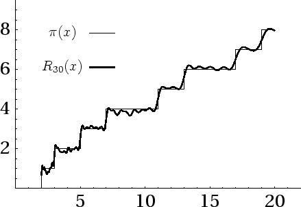
all the nontrivial zeros of the zeta function have real part equal to .

This has been checked into the millions - that is, that all the zeros with imaginary part into the millions and in the critical strip are actually on the line

In order to relate $\zeta(s)$ to $\pi (x)$ Riemann defined a weighted prime-counting function

$\begin{displaymath}\Pi(x) = \sum_{p^m\leq x}{1\over {m}}{ }.\end{displaymath}$

In other words, whereas $\pi (x)$ is a step function that adds one for every prime, $\Pi(x)$ is the step function that adds $1\over m$ for any power of a prime .
Note that $\pi (x)$ and $\Pi(x)$ are step functions whose value at a jump point, when graphed, is the height of the upper point. For the following discussion we redefine these functions to have value at a jump point the average of the height of the lower and upper points of the jump.

The function $\Pi(x)$ can be obtained from $\pi (x)$ by the infinite series:

$\begin{displaymath} \Pi(x) = \sum_{n=1}^\infty\frac{1}{n}\pi(x^{\frac{1}{n}}) \end{displaymath}$

(1)

This equation, in turn, can be inverted to compute $\pi (x)$ from $\Pi(x)$ as

$\begin{displaymath} \pi(x) = \sum_{n=1}^\infty \frac{\mu(n)}{n}\Pi(x^{\frac{1}{n}}) \end{displaymath}$

(2)

where $\mu(n)$ is the Möbius function which is

is divisible by a prime square,

is a product of an even number of distinct primes and

is a product of an odd number of distinct primes.
Riemann showed that $\Pi(x)$ can be determined from the zeros $\rho$ of the zeta function by the equation

$\begin{displaymath} \Pi(x) = Li(x) - \sum_{\rho}Li(x^{\rho})-\log(2)+\int_{x}^{\infty}\frac{dt}{t(t^2-1)\log(t)}\;\;\; (x > 1) \end{displaymath}$

(3)

Here the sum on $\rho$ in the second term is taken with increasing values of the absolute value of the complex part of $\rho$ .
Putting (3) into (2), $\pi (x)$ can be determined from the zeros of the zeta function. For fixed x, (2) is a finite series. Thus if we use the first k zeros of the zeta function in (3) we will obtain an approximation to $\Pi(x)$ .

**Figure 2:** Approximating $\pi (x)$ using the first 30 zeros of the zeta function. Click here for an amusing animation using the first 500 zeros. And clickhere for an animation of $\pi (x)$ being approximated in the interval $190 \leq x \le 230$ , again using the first 500 zeros.
$\begin{figure}\begin{center} \epsfig{figure=pivsrAll.eps,width=0.8\textwidth}\end{center}\end{figure}$

So, as we use more and more of the zeros of the zeta function we eventually get a good approximation to the number of primes less than or equal to x. In the limit we would get the exact value.

Hans Riesel and Gunnar Göhl [2] show how these computations can be carried out. We illustrate this approximation in Figure 2. The animations show how the approximation improves when we increase the number of zeros used.

Riemann's proof of formula (3) was not complete and a rigorous proof was first provided by H. von Mangoldt.

The function $\Pi(x)$ introduced by Riemann has pretty much been replaced, in modern studies of prime numbers, by a similar function $\Psi (x)$ , introduced by Chebyshev, a Russian mathematician famous for making some of the first progress on the Prime Number Theorem and also for having a seemingly infinite number of accepted spellings of his name.

$\Psi (x)$ is again a step function which starts at 0 but now has a jump of $\log(p)$ at each prime power . Thus

$\begin{displaymath} \Psi(x) = \sum_{p^n < x}\log(p) \end{displaymath}$

(4)

We redefine $\Psi (x)$ at jump points in the same way we did for $\pi (x)$ and $\Pi(x)$ .

**Figure 3:** Comparing and $\Psi (x)$ .
$\begin{figure}\begin{center} \epsfig{figure=chebyPsiAll.eps,width=0.7\textwidth}\end{center}\end{figure}$

Chebyshev proved that the prime number theorem is equivalent to the statement that $\Psi(x) \sim x$ . (See Figure 3). And knowing the error in using the approximation of for $\Psi (x)$ is equivalent to knowing the Error term for our approximation to $\pi (x)$ .
The Riemann Hypothesis has been shown to be equivalent to the following estimate for the difference between $\Psi (x)$ and :

$\begin{displaymath}\vert\Psi(x) - x\vert \le cx^{1/2}(\log x)^2\end{displaymath}$

for $x\ge 2$ .
Mangoldt showed that $\Pi(x)$ can also be determined from the zeros of the zeta function by the following equation:

$\begin{displaymath} \Psi(x) = x - \sum_{\rho}\frac{x^\rho}{\rho} - \frac{1}{2}\log(1-\frac{1}{x^2})-\log(2\pi) \end{displaymath}$

(5)

Again the sum is taken in increasing order of the absolute value of the complex part of $\rho$ . Thus, using the first k roots $\rho$ of the zeta function, we can obtain from equation (5) an approximation for $\Psi (x)$ . We illustrate this approximation in Figure 4 and again the animations show how the approximation improves when we increase the number of zeros used.

**Figure 4:** Comparing $\Psi (x)$ with its approximation via summing the first 50 zeros of the Zeta function. Click here for an animation! Animations are also available for views of $\Psi (x)$ being approximated in the interval $2\frac{1}{2} \leq x \le 5$ : a slow one using the first 100 zeros, and a fast one using the first 500 zeros.
$\begin{figure}\begin{center} \epsfig{figure=psiApproxAll.eps,width=0.8\textwidth}\end{center}\end{figure}$

Thus the product formula for $\zeta(s)$ suggests that that the zeta function knows the prime numbers and formulas (3) and (5) suggest that the zeros of the zeta function know the distribution of the prime numbers.

Dan Rockmore's story "The Chance of a Prime" will be continued in future issues of Chance News.

References

[1] H. M. Edwards, Riemann's Zeta Function, Dover Publications, 2001.

[2] Hans Riesel and Gunnar Göhl, "Some Calculations Related to Riemann's Prime Number Formula,'' Math. Comp. 24 (1970), pp. 969-983.

The are numerous web sites devoted to prime numbers and the Riemann Hypothesis. Just search on Google using "prime numbers'' or "Riemann Hypothesis."

About this document ...

Peter Kostelec 2001-12-10