!!!!!!!!!!!!!!!!!!!!!!!!!!!!!!!!!!!!!!!!!!!!!!!!!!!!!!!

      CHANCE News 10.09

   September 19 , 2001 to October 29, 2001

!!!!!!!!!!!!!!!!!!!!!!!!!!!!!!!!!!!!!!!!!!!!!!!!!!!!!!!

Prepared by J. Laurie Snell, Bill Peterson, Jeanne Albert, and Charles Grinstead, with help from Fuxing Hou and Joan Snell.

We are now using a listserv to send out notification that a new issue of Chance News has been posted on the Chance website. You can sign on or off or change your e-mail address at this Chance listserv. This listserv is used only for mailing and not for comments on Chance News. We do appreciate comments and suggestions for new articles. Please send these to:

jlsnell@dartmouth.edu

The current and previous issues of Chance News and other materials for teaching a Chance course are available from the Chance web site.

Chance News is distributed under the GNU General Public License (so-called 'copyleft'). See the end of the newsletter for details.

Why Bonds won't break the homer record
and the placebo effect might be bunk.

Jordan Ellenberg,
Slate, 12 July, 2001

In statistics, never say never.

Laurie Snell

Contents of Chance News 10.09

1. The Probability/Statistics Object Library.

2. A Dilbert Cartoon.

3. A candidate for Forsooth.

4. A study links prayer and pregnancy.


5. Car Talk boys rant and rave about GM study.

6. Publications ethics: Truth or consequences.

7. Reckonings: An injured city.

8. Marilyn vos Savant on the average losses of a typical visitor to a casino?

9. Are high school athletes more likely than their peers to graduate from college?

10. Return to population growth and tricky graphs.

11. Curve Ball: baseball, statistics, and the role of chance in the game.

12. A major study with a small n.

13. The World of Chance: a chance course.

14. A role of statistics in international cricket.

15. Using songs in teaching statistics.

16. Lewis Carroll's obtuse problem.

Kyle is now developing, under an NSF grant, a new resource called The Probability/Statistics Object Library. In this library you will find statistics and probability applets and their components. If you would like an applet you are invited to add it to your own web page and to write your own text relating to it. For example, we added Kyle's Sample Mean applet to this web page to show how this works. The components of the applets are made available to help students and teachers (who have some programming experience) to make their own applets.

Kyle has put his Object Library under the GNU contract which makes the applets and their components freely available with the source to encourage others to make improvements which also will be freely available to all. This idea of "open software" has had some spectacular successes in computing, most notably Linux, and it would be nice if this project were to lead to a combined effort to produce interactive materials for teaching probability and statistics.

Dilbert Cartoon, 25 October, 2001.
Scott Adams

In this cartoon the Director of Accounting is giving Dilbert a tour of accounting.

The Director: Over here we have our random number generator

The Director: NINE, NINE, NINE, NINE, NINE, NINE

Dilbert: Are you sure that's random?

The Director: That's the problem with randomness. You can never be sure.

Here is a candidate for Forsooth:

In an article "Measure of inflation for home run race, New York Times, 30 Sept 2001, sports desk, by Murray Chass we read:

The idea of anyone hitting 338 home runs in a season is silly,
but that's the number of home runs Babe Ruth would have
this season if he had come back and produced the same ratio
of home runs he accounted for in 1927.

Chass says further

When Ruth hit 60 in 1927, his output represented 6.5 percent of the home runs
hit in the major leagues. ...Bonds, with 69, has produced 1.3 percent of the home
runs this season. Bond's ratio was one-fifth of Ruth's, which explains the 338
home runs Ruth would have this year based on his 1927 ratio.

DISCUSSION QUESTIONS:

(1) How do we get 338?

(2) What facts about the difference between major leage baseball in 1927 and in 2001 would have to be taken into account to make this comparison have any meaning?

Vital signs: fertility; a study links prayer and pregnancy
The New York Times, October 2, 2001
Eric Nagourney

Does prayer influence the success of in vitro fertilization-embryo transfer? report of a masked, randomized trial.
Journal of Reproductive Medicine, Vol.46, No. 9 (September, 2001)
K.W. Cha, D.P. Wirth, R.A. Lobo

According to the journal article, the objective of the study mentioned in the title is to "assess the potential effect of intercessory prayer on pregnancy rates in women being treated with in vitro fertilization-embryo transfer (IVF-ET)." Intercessory prayer is defined to be a request for "God's intervention or assistance for the benefit of another individual." (People engaged in such prayer are called "intercessors".) The Times article is a brief summary of the results.

During the study three different prayer groups were formed: some individuals prayed directly that women who were undergoing IVF-ET procedures would have increased pregnancy rates, while others prayed that these people's prayers would be more effective. A third group "prayed in a general, nonspecific manner with the intent that God's will or desire be fulfilled." Treatment (women prayed for) and control (not prayed for) groups were followed through the IVF-ET process and the prayed-for group had double the pregnancy rate (44/88 versus 21/81).

The article states that patients were stratified based on age, length and type of infertility, and number of prior attempts before being randomly assigned to treatment or control groups. A fairly elaborate double-blind scheme is described for assigning intercessors to patients, along with a comparison of several important stages of pre-embryonic development for women in the two groups. The crucial difference in outcomes between the groups appears to be at the embryonic transplantation phase of the process. Given the controversial nature of the research, it is surprising that there is virtually no discussion of whether the stratification process might have failed to identify the sort of fertility problems that would lead to such a difference in rates. Although the authors note in the journal that they "are highly cognizant of multiple unknown variables, which might affect pregnancy rates", they also state that "randomization took into account such variables as type of infertility."

DISCUSSION QUESTIONS:

(1) Which do you think is more likely and why: that prayer contributed to the improved pregnancy rates of the treatment group, or that a hidden but significant difference between the treatment and control groups contributed to the difference in rates?

(2) The patients and health care providers were unaware that they were part of the study. Why do you think this was done? Do you think it was the right thing to do?

(3) In the Times article one of the authors (Lobo) mentions his initial reluctance to publish the results. Do you think this article should have been published? Why or why not?

Risk is one in four Million? I beg to differ.
Car Talk, Rant and Rave, 20 October 2001
Tom Magliozzi

Association between embedded cellular phone calls and vehicle crashes involving air bag deployment.
Richard A. Young, General Motors

The Car Talk guys have a "rant and rave" feature of their NPR program. In a rant and rave written by one of the brothers, Tom Magliozzi, Tom ranted and raved about the absurdity of a GM cellular phone study. He said it was completely bogus and suggested that GM intended to deceive the public. After receiving a letter from the GM legal affairs department, the brothers removed this rant and rave from the Car Talk site and, on the October 20 program, they apologized to GM for being so hard on its study. They also provided a new version of their rant and rave report on this study. This revised rant and rave was toned down a bit but the substance of their criticism, which we will report below, has not changed in this new version.

For the last five years, GE has included a feature called "OnStar" on many of their models. OnStar provides an "embedded" cell phone that allows the driver to make calls by listening and speaking using a built-in microphone and speaker allowing the driver to keep his hands on the wheel.

Beside making ordinary calls, the driver can push a button connecting to a service advisor who will answer questions about directions, getting help with car problems, etc. Also, if the driver has an accident that causes an air bag to be deployed, the OnStar system automatically places an "air bag call" to an advisor who will then try reach someone in the car and, if this fails, will call for help. Recently, GM has introduced a "virtual advisor" that will allow the driver to get traffic information, internet information such as e-mail messages, stock information,etc.

The author of the GM study,Young, writes in his introduction:

There are more than 100 million portable cellular phone owners
in the United States and 73 percent of them report using their phone
while driving. At the same time, there has been a lack of accurate
real-world scientific data to analyze cell-phone use in vehicles and
its relationship to crashes. Laboratory studies purporting to reach
conclusions about real-world driving rarely report validating their
methods or findings with on-road testing, leaving generalizations
to real-world driving speculative at best. The few real-world studies
to date make only statistical inferences from small samples in limited
geographic regions. Also, the crash times recorded by observers at
crash scenes may not be accurate or synchronized well with call times
recorded by cellular telephone service providers. Therefore, it has not
been possible to determine accurately which came first, the call or the
crash. A random error of even a few minutes in estimating the time of
a crash may overestimate the number of calls before the crash, because
of misclassification of calls after the crash.

These remarks suggest that the GM study is aimed at avoiding these problems and to estimate the safety of the use of cell phones in real-world driving .

The GE study looked at the 8- million OnStar calls that advisors received over the five-year period from October 1996 to May 2001. It was found that, in these 8-million calls, there were only eight cases of OnStar voice conversations followed in less than 10 minutes by an air bag call. The advisor's written comments suggested that only two of these phone calls extended to the time of the crash. From this it was concluded that:

(1) An embedded cell-phone call with an advisor followed by air bag-deployment crash within 10 minutes occurred at a frequency of one event per million calls.

(2) an embedded cell phone in use at the time of an air bag-deployment crash occurred at a frequency of one event per 4-million calls.

Tom starts his rant and rave by observing that GM has restricted accidents to those in which an air bag is deployed. He remarks that air bags deploy only if a car is involved in a frontal accident that occurs above approximating 25 to 30 mph and estimates that this is only 5 percent of the accidents. (In his original rant and rave he estimated 1 percent, which he said was based on data from the National Highway Traffic Safety Administration.) Thus to take into account all accidents we should multiply the numbers 2 and 8 by 20 giving an estimate of 40 accidents in which the cell phone was used at the time of the accident and 160 where it was used within ten minutes of the time of the accident.

Next Tom observes that in the five-year period of the study about 130 billion cell-phone calls were made. Of this he assumes that 50 percent were made while in moving cars. He remarks that he does not think that the real percentage is known. (in the earlier rant and rave he said: Thanks to the Yankee Group, a research company in Boston, we know that about 65 percent of all cell-phone calls in 2000 were made while in transit.) Assuming the 50 percent figure this means that there were 65 billion calls in transit. Thus the 8 million OnStar calls represent .012 percent of the calls made. Therefore, our estimate of 40 accidents for which the cell phone was used at the time of the accident extrapolates to 320,000 accidents and the 8 for which the cell phone was used within ten minutes of the accident extrapolates to a whopping 1.28 million accidents during this five year period. Now the use of cell phones does not seem so harmless.

Finally Tom observes that the OnStar calls are not representative of cell-phone calls generally. The caller is talking to an advisor trained to speak in a calm and friendly manner in contrast to calls from the driver's boss asking where his report is or from his wife asking why he is late for dinner etc.

Tom then mentions that several recent studies have shown that driving while using cell phones is dangerous and writes:

So, if you'er like us, you're left wondering: Why would GM publish the results of this study? Well, funny you should ask. It just so happens that GM is at the forefront of "telematics," the technology that will bring yet more distracting features to your car. They stand to make hundreds of millions of dollars with e-mail, Web access, and cell-phone technology in its new cars.

DISCUSSION QUESTIONS:

(1) At the end of the GM study we read:

The data in the current study is based on a census of tens of thousands
of vehicles and millions of calls. There are no statistical projections or resulting sampling errors in the data; the confidence intervals on the results are all zero (no errors). What does this mean?

(2) What do you think about Tom's critique of the study?

Publication ethics: Truth or consequences.
The Economist, 15 September 2001, 70-01.

This is a follow up to a story from the last edition of Chance News. There we reported that editors of biomedical journals had issued new policies to prevent corporate sponsors from withholding data from investigators or restricting publication of unfavorable research findings.

The Economist argues that outside money is not the only source of bias in published research. According to the article, existing publication guidelines indicate that authors listed on a paper should have contributed to the study's design, the data analysis and the written presentation. This all seems to make sense. But when the British Medical Journal analyzed 129 submitted articles with a total list of 588 authors, not all of the authors met the standards. Depending on how strictly the guidelines were interpreted, compliance was between 24% and 71%.

The editor of the Lancet, Richard Gorton, took a different tack, asking whether the conclusions reached in published articles reflected the views of the authors listed. Of course, it is unrealistic to expect perfect agreement on all points. However, Gorton found an unfortunate trend: the contributor with the most to gain from the publication was often able to suppress the legitimate criticisms of co-authors.

An investigation by the Citroen Corporation, a group which studies clinical trials, found that reports of experiments in the leading journals do not adequately review the literature for results of related trials. For example, of the 33 trials published in May of this year, none compared its results to earlier experiments--and four erroneously claimed to be the first research done in their area!

DISCUSSION QUESTION:

The article notes that, in principle, many of these problems ought to be caught prior to publication by the peer review process. Can you think of reasons why they might not be?

What will be the long term effects of September 11 on New York's status in the American economy? Krugman points out that the city's historical advantages, such as its water ports, are less relevant today. Businesses continue to locate in New York largely because of the presence of other businesses there. Krugman wonders whether the terrorist attacks will lead some businesses to leave the city. This would depress the economy, potentially causing more business to leave, thus causing further economic decline. Such a feedback cycle could conceivably destroy the city's economic viability.

Of course, Krugman observes, one cannot conduct experiments on cities to test such a theory. But, coincidentally, two Columbia University professors have recently published a paper entitled "Bones, bombs and break points: The geography of economic activity", which considers the results of the US bombing of Japan at the end of World War II. Some cities were almost entirely destroyed, while others suffered relatively little damage. (On a percentage basis, the area destroyed in Tokyo was about average for all cities.) Yet despite this wide variability in damage, Japan's cities recovered quickly after the war to assume their former rankings in the overall economy.

Krugman sees this as evidence of "the robustness of cities." He concludes that "if the Japanese parallel is at all relevant, the attack on New York, for all its horror, will have no effect worth mentioning on the city's long-run economic prospects."

DISCUSSION QUESTIONS:

(1) What differences do you see between the Japanese example and the current situation in New York?

(2) Can you think of any historical counterexamples to the robustness principle described here?

A reader asks: "What are the average winnings or losses of a typical visitor to a casino?"

After noting that casinos "are the winners every day," Marilyn says that on average visitors lose 5.3% of their money when they play the slot machines, and 14.17% when they gamble at tables.

DISCUSSION QUESTION:

Marilyn gives enough significant digits to suggest she has some very specific data in mind. What do you suppose these figures represent?

Morin challenges the conventional wisdom about the benefits of high school sports. Previous studies have found that varsity athletes are more likely to go to college, where they are more likely to graduate and ultimately earn more money that their peers who didn't play high school sports.

But Eric Eide of the RAND corporation has found that these conclusions do not hold up uniformly when the data are broken out by gender or race. It turns out that white male high school athletes are actually less likely to graduate from college. And while white female athletes are more likely to attend college and graduate, they do not enjoy superior earnings later in life. The greatest benefit was observed for black males athletes, who do fare better in college and later employment.

Eide's study used data collected over the last two decades by following 10,000 men and women who were high school sophomores in 1980. His analysis is published in the journal "Economics of Education Review."

DISCUSSION QUESTIONS:

(1) The article notes that Eide's analysis "did not produce precise estimates of how much more black male high school athletes earn later in life, or exactly how much playing sports increases their chances of going to college or graduating--only that playing sports helps in both categories." What do you think this means? (Were the differences not statistically significant?)

(2) When studying future earnings, is the comparison made for graduating athletes vs. non-athletes, or all athletes vs. non-athletes? Does it matter?

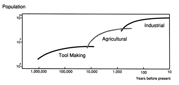
In Chance News 10.05 we discussed an article in the May-June issue of the American Scientist by Peter Schulze and Jack Mealy called "Population growth, technology and tricky graphs." Because we were sending Chance News by e-mail we could not include graphics. Thus it was hard to show what the authors were concerned about in this article. We can now include the relevant graphs and make this clearer.

The article was centered on a graph charting the history of the world population that appeared in an article by the famous ecologist Edward S. Deevey Jr. in the September 1960 issue of Scientific American. The graph in question is the following loglog plot of the world population back a million years:

Recall that such a loglog plot plots the logarithm of years against the logarithm of the population. Schulze and Mealy reamrk that this graph appeared in several articles and books and has been used to argue that the population tends to level off in major periods of human evolution. For example, it appears in the recent book "Human Impact on the Earth", William B. Meyer, Cambridge University Press, 1996 where we read:

A possibility that this picture raises is that each great transformation of society may raise the globe's human carrying capacity to some new plateau. Population rises to that height and stabilizes; what happened twice in the past may happen again.

To show that loglog plots are deceptive in this application, Schulze and Mealy ask: What sort of growth would be neeeded to show an obvious increase on a graph with two logarithmic axes? They write:

To rise as a straight line, a variable must make its next order
of magnitude increase in an order of magnitude less time than
the previous one. For example, consider a population that went
from 100 to 1,000 in 100 years, an annual increase of 2.33
percent. To plot as a straight, upward-sloping line, the population
would have to reach 10,000 in the next 10 years and then hit
100,000 in the following year. No population of organisms could
long keep up such accelerating multiplication. So regardless of
the actual situation, all plausible positive rates of growth will appear
to plateau on Deevey's graph.

Peter Schulze sent us the data that was used in trying to reconstruct the Deevey graph. Hear it is:

Of course, data back a million years ago cannot be expected to be very accurate. Different researchers have provided different numbers. You can obtain this data in Excel format and references that Schulze and Mealy used here. Similar estimates are provided here by the census bureau.

We used this data to try to reproduce the Deevey graph. Here is the result:

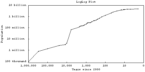
Obviously, we cannot expect a smooth curve when we have so little data from the early years. Apparently, Deevey smoothed his curve to make it look more attractive.

Since we have seen that this graph is deceptive, how should we plot the world population to see what is going on? The most straightforward method would be to use arithmetic scales. If we do this we obtain the graph:

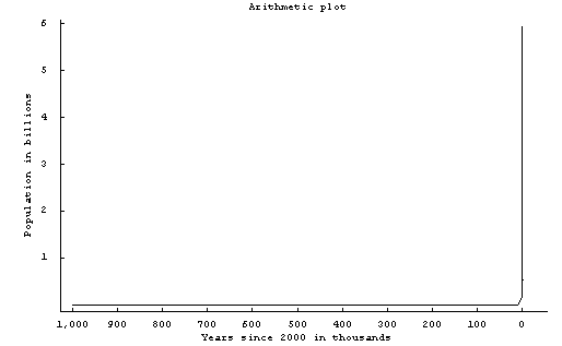
While not a very interesting looking graph it does that population increased dramatically in a relatively short period. However, it does not show much detail for either before or after this population explosion.

One of the principle sources of early estimates of the population is the "Atlas of World Population History" by Colin McEvedy and Richard Jones, 1998, Penquin, New York. Here is how the world population is plotted from 400 BC to 1975.

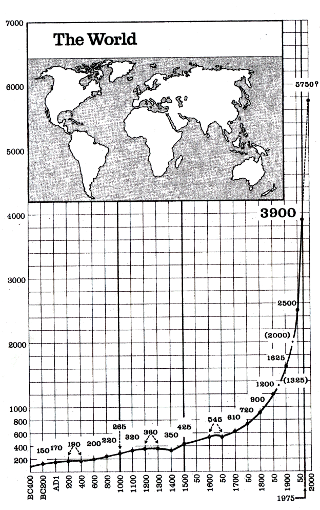
The time period and used an arithmetic scale for the population they use their own scaling for the time axis. Their data is on the graph. We see only one population decrease which occurred between 1300 and 1400 AD. This decrease was the result of the Black Plague. It was estimated that as many as 25-million people in Europe died as a result of this plague.

This graph includes Deevey's industrial period and a good part of his agricultural period. There is certainly no evidence of the population leveling off in either period. Also we note that the authors' prediction, made in the 1970's, that the population in 2000 would be 5,750,000,000 was a pretty good estimate since the world population in 2000 was 6,080,000,000.

Since in population changes it is reasonable to assume that the rate of growth of the population should be proportional to the number of people alive, we should expect the growth to be exponential. If that is the case a log plot would enable us to see the rate of growth. Here is such a log plot for the industrial period.

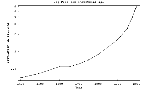
We would expect a straight line if the population increased at a constant rate. The graph suggests that this approximtely true until 1600. But after 1600 it increased at an increasing exponential rate.

What about the future? The census bureau gives us predictions up to the year 2050. They provide us with a graph of the population from 1950 projected to the year 2050:

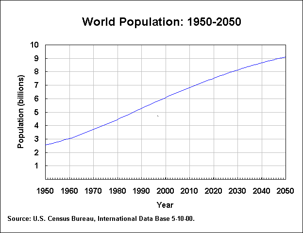
We see that the Census Bureau predicts that in the next 50 years the rate at which the populations grows will decrease. However it will still increase to about 9 billion by 2050.

George Cobb wrote an interesting commentary on the Schulze-Mealy article and on the use of log plots as a letter to the editor in the July-August 2001 issue of the American Scientist. Readers will enjoy reading his commentary and the reply by Schulze and Mealy.

DISCUSSION QUESTION:

Do a search on "log plots stocks dow" and comment on the use of these plots in the analysis of trends in stock prices and stock indices.

Curve Ball: Baseball, Statistics, and the Role of Chance in the Game.
Copernicus Books, 2001
Hardcover, 369 pages, List price $29, Amazon $20.30

At the Joint Statistics Meetings in Atlanta this summer there was a session on teaching an elementary statistics course based on the statistics of baseball. The speakers were aware that this might not be everyone's cup of teach but said that they did this in a setting where students had other choices for their first statistics course. Their courses all sounded great. One of the speakers was Jim Albert from Bowling Green State University. Jim wrote this book with Jay Bennett and it provides a great text for such a course. It is also a wonderful book for any baseball fan who wants to look beyond the numbers to appreciate the subtleties of the game and the role that chance plays in it.

The popular idea of a sports statistician is of one who collects all kinds of data and provides them to sports announcers to liven up their broadcasts, while we think of a statistician as someone who collects data and analyses it A student who likes baseball and takes a course with this book as text will have an opportunity to see the power of statistical analysis as it relates to something he or she really cares about.

The authors follow the current trend of avoiding complicated mathematical discussions, using simple experiments involving coin tossing, spinners, and computers to simulate complex experiments. Their approach is to identify an interesting question and then show how statistics can help solve it. We describe one simple example to illustrate this approach.

We are told that Scott Rolen came to bat 601 times in 1998 and got 174 for an observed batting average of .290. The authors use a simple spinner model to simulate Scott Rolen's season performance, assuming that he has a true batting average of .300. By simulating a hundred seasons, the students see considerable variation in the observed batting averages. A stemplot of a 100 seasons suggests a bell-shaped curve.

The authors then find the batting averages for the 246 players in 1988 who came to bat at least 300 times. Plotting these, again using a stemplot, results in a bell-shaped curve with averages clustering in the range 250-299 with median value .276.

The authors then consider two different models for batting averages. In the first model a players' hits are simulated by a .276 spinner model corresponding to each player having the same true batting average. For the second model, the players' batting averages are chosen at random from the bell-curved distribution obtained from the 246 players in 1988.

Using the first model to simulate the batting averages for the 246 players in one season, the authors show, by a box plot, that there is signficantly less variation in the .276 model than in the actual batting averages. Simulating the batting averages using the second model results in a stemplot very similar to that of the actual batting averages, showing that players with different batting averages is a better model.

Of course the students will not be surprised by this result, But now they will be prepared to use similar methods to investigate the more interesting problem of whether different situations, such as play at home vs. away, playing in the daytime vs. night, playing on grass vs. turf, make a significant difference in players' batting performances.

A still more difficult problem is the problem the authors call "the great quest" described as:

What is the best formula for evaluating offensive performance? Who
is the more valuable player, a Tony Gwynn type of hitter, who has a
high batting average but little power? or a Mike Schmidt type, who
displays great power but has a low batting average? And just how
valuable is speed in a player? or the ability to draw a walk? Or..

Here the student learns that considerable progress on this quest can by made by applying standard statistical techniques, such as regression, which have nothing to do with baseball in particular. The authors make interesting comparisons between the results of using statistical methods with results of baseball experts who have used their own intuitive methods based on years of studying baseball.

Of course we also find a chapter on streaks in baseball. Here again simulation is the basic tool. The authors define Mr. Consistent to be a player who gets a hit with the same probability each time he comes to bat. Mr. Streaky is a player who in each game is hot (probability .380 of getting a hit each time at bat) or cold (probability .180 of getting a hit each time at bat). If the player is hot in one game he will be "hot" in the next game with a probability s and if he is cold in one game he will be cold in the next game with probability s with s > 1/2.

Individual players' performances are compared against each of these models to see if streaky behavior stands out. The authors use moving averages and runs tests for this comparison. They show the necessity of looking at large amounts of data to avoid selection bias. When they do this they do not find evidence of streaky behavior but, at the end of the chapter, they confess their own feelings based on their experience playing which are based on their experience playing Little League basketball in their youth:

On some days we would feel that we had the right shooting touch
and could make any basket we would try. On those days we believed
we had a true hot hand--our shooting stroke had just the right rhythm
so that we had a high probability of making a shot. Other days, we
would be out of rhythm and have little feeling for the location of the
hoop--we would have a much smaller probability of aiming a shot.
So a hot hand refers to a feeling -- it's an intrinsic characteristic of
our shooting ability.

Norton Starr suggested the following letter to the editor in the New York Times.

On the bioterror front: fear and vigilance.
New York Times, 24 October 2001, A20, Letter to the editor
Peter Lurie

You quote Tommy G. Thompson, the secretary of health and human
services, as saying "doxycycline and penicillin are just as effective as
Cipro" (news article, Oct. 20). The major study in the field, published
by United States Army researchers in 1993, does not support this
statement.

In that study, groups of 10 monkeys received either doxycycline,
ciprofloxacin, penicillin or placebo for 30 days, beginning one day
after exposure to a large inhaled dose of anthrax. Although no
treated animals died from anthrax by Day 30 (compared with
nine in the placebo group), in the 30 days after stopping treatment,
one animal in both the ciprofloxacin and doxycycline groups died
from anthrax, compared with three that received penicillin.

Moreover, the penicillin was injected, while the other antibiotics
were taken by mouth.

Based on these data for this strain, were we exposed to anthrax,
we would take ciprofloxacin or doxycycline, but not penicillin.

Peter Lurie, M.D.
Sidney M. Wolfe, M.D.
Washington, Oct. 20, 2001

DISCUSSION QUESTION:

Do you think that this study was large enough support Lurie's recommendation?

We found a number of interesting articles while browsing through the last two issues of Teaching Statistics. Incidentally, our library does not have the hard-cover version of Teaching Statistics, and we were surprised to find that it does have the electronic version as part of a package deal with Blackwell publishers through the distributor ingenta. If your library does not get a hard cover version of Teaching Statistics you might want to check to see if they have the electronic version. Curiously, we were told by Blackwell that you cannot get the electronic version if you have a personal subscription to the journal.

The World of Chance.
Teaching Statistics, Vol.23, No.2, Summer 2001, 61-64
Alice. M. Richardson, University of Canberra, Australia
alicer@ise.canberra.edu.au

While the Dartmouth Chance course has thrived for the past ten years, we are not aware of very many schools that are teaching a Chance course.. Thus it is great to read Professor Richardson's account of teaching such a course since 1999. Her article describes how she teaches the course--- what has worked and what has not worked-- and provides a wonderful list of resources and references. You can see details of her current version of The World of Chance at the course website You will see from the syllabus that there is a significant unit on good and bad graphics. Also, Professor Richardson makes good use of visiting lecturers something that we always found useful in our Chance course. From her current syllubus we find:

There will be two guest speakers in the lectures in Week 11: Professor John Croucher of the Department of Statistics at Macquarie University will be speaking on the statistics of gambling, and Dr Ann Cowling of the Statistical Consulting Unit at ANU will be speaking on distance sampling.

Professor Richardson has provided us with a copy of an article that was the basis for the Teaching Statistics article. You can find this article here. The fonts may not look good on the screen, but if you print it out it will be fine. One interesting thing that is in this article and was in the Teaching Statistics article is the results of surveys of the students on their attitudes about statistics given at the beginning and at the end of the course.

Professor Richardson's ends her account of her course with:

If anyone reading this is contemplating getting involved in the
world of Chance, I would strongly recommend getting hold
of the resources described, keeping an eye on the news for
up-to-the-miute examples and having a go!

To which we say Amen!

A role of statistics in international cricket.
Teaching Statistics, Vol. 23, No 2, Summer 2001, 39-43
Frankk Duckworth

Pascal and Fermat's solution of the problem of how to divide the stakes when a best of n series has to be discontinued before the series is completed is given credit starting modern probability theory. This article tells the story of how Frank Duckworth and Tony Lewis solved a similar problem of determining the winner when a cricket game has to be discontinued because of rain.

The method has become known as the D/L method and has been put into use in major cricket competitions worldwide.

Frank is a good story teller and he has an interesting story to tell.

DISCUSSION QUESTION:

Can you name any other work of a sports statistician that has affected the outcome of a game?

Musical means: using songs in teaching statistics.
Teaching Statistics, Vol. 23, No. 3, Autumn 2001, 81.84
Lawrence M. Lesser

This article suggest that we should take advantage of our students' love of music to motivate studying statistical concepts. Here are a few of Lesser's suggestions:

Surveys on student preferences can be carried out and analyzed. Tests of hypotheses can be carried out to test if more than 50% of the hits are co-authored, written in a major key etc. Lesser shows how statistics in lyrics can also be used to start interesting statistical discussions. Our own favorite is the line in a lyric by Canadian rock band Rush (1981):

Random sample, hold the one you need.

Lesser also gives examples where permutations and combinations arise naturally is answering questions such as how many melodies can result from Mozart's famous "Musical Dice Game"?

Finally Lesser invites us and our students to come up with new example of statistics in music.

Lewis Carroll's obtuse problem.
Teaching Statistics, Vol. 23 No. 3, Autumn 2001
Ruma Falk and Ester Samuel-Cahn

It is said that Lewis Carroll wrote his famous Pillow Problems at a time when he was having trouble sleeping. His problems were published in 1895 and are available today in the 1958 Dover book "Pillow Problems and a Tangled Tale".

One of Lewis Carroll's problems was:

Three Points are taken at random on an infinite Plane. Find the
chance of their being the vertices of an obtuse-angled triangle.

Falk and Samuel-Cahn provide Carroll's solution to this problem which resulted in his answer:

Probability angle is obtuse = 3pi/(8pi - 6sqrt(3)) = .6394

They then point out that the Carroll assumed the existence of a triangle resulting from choosing three points at random from the plane. Of course, we know that there is no way to choose a point at random from the plane in standard probability theory, so one should not be surprised to find that this solution cannot be defended. To demonstrate this they derive a different answer starting with the same assumptions that Carroll made.

They then raise the question of what the answer would be if you chose the points from a finite region of the plane. They point out that only the shape of the region matters, not its size. They first consider choosing a random point in a square. They suggest that finding an analytic solution is hard, so they use simulation. They obtain an answer of approximately .7249 using a million simulations. For a circle, again, by simulations they get the answer .7201. They also consider rectangles and equilateral triangles.

After they did their work the authors learned that the exact answer for the square had been obtained by E. Langford in "The probability that a random triangle is obtuse", Biometrika 56 (1969) 712-5, and for the circle in G. R. Hall's paper "Acute triangles in the n-Ball", Journal of Applied Probability 19 (1982) 712-5. For the square the probability the triangle is obtuse is

Probability angle is obtuse = 97/150 + pi/40 = .7252...

and for a circle it is:

Probability angle is obtuse = 7/8 - 4/pi^2 = .7197...,

so the authors simulated values are consistent with these results.

Thus if we were to try to define the original problem as the limit of finite regions going to infinity, we would get different answers depending on the nature of the finite regions we chose.

DISCUSSION QUESTION:

Why does the answer depend only on the shape of the region?

We have discussed only two articles from each of the last two issues of Teaching Statistics. There are many more interesting articles. You can see the table of contents of the current and previous issues and learn more about this journal at the Teaching Statistics homepage.

Copyright (c) 2001 Laurie Snell

This work is freely redistributable under the terms of the GNU
General Public License published by the Free Software Foundation.
This work comes with ABSOLUTELY NO WARRANTY.

!!!!!!!!!!!!!!!!!!!!!!!!!!!!!!!!!!!!!!!!!!!!!!!!!!!!!!!! !!!!!!!!!!!!!!!!

CHANCE News 10.09

September 19, 2001 to October 29, 2001

!!!!!!!!!!!!!!!!!!!!!!!!!!!!!!!!!!!!!!!!!!!!!!!!!!!!!!!!!!!!!!!!!!!!!!!!!!